basilh@virginia.edu
@basilhalperin
This fall was my first time teaching – one class, undergrad intermediate macro, with 60 students.
(While I did many stints as a teaching assistant during grad school, being the professor I think is a bit of a different beast. You’re ultimately responsible!, and you have to hold a lot more in your head at once. There’s a lot more that could be said – and that I hope to say in the future – on the experience of teaching, and also on how I taught intermediate macro in particular. But that’s not today’s post.)
Before the start of the semester, I decided to put together a list of “principles of teaching” to try to guide my teaching efforts. Because teaching is such a high-dimensional design space – when you start teaching, you are really given an extreme, an extraordinary level of freedom to do whatever you want – I wanted some points to anchor to.
Below, I start with some brief thoughts on the goals of teaching. Then, I list the principles for achieving those goals, plus some references/selected quotes that inspired each (the principles mostly drew on the experience of others). I‘ll hide all but the very best quotes below the clickable arrows – but I do recommend opening and reading the quotes.
I think of four goals of teaching:
An alternative framing is that there are two populations when teaching, and I’m aiming for different treatment effects on each:
The extent to which students find themselves in the tail versus in the mass is of course endogenous – aiming to inspire is important for affecting this!
0. Have extreme empathy. Honestly, I think quite literally everything is downstream from this.
1. Grading should be predictable. This is a boring one to start – it’s not about actual learning – but of course, from the perspective of the student this is pretty central.
2. Enthusiasm matters! Show that you care – channel your enjoyment! This reflects both that teaching is an entertainment service; and it reflects the goal of inspiration. Tyler Cowen puts this fantastically well:
3. Actively solicit feedback. This is one of those things that is obvious but maybe not obvious if you’re not intentional about it.
(i) David Cutler: “Whenever students talk to me outside of class, I always ask them how the course is going.”
(ii) Besides the benefits for teaching itself, students themselves directly value the opportunity to have voice.
(iii) Obviously, receiving feedback may be painful; and feedback may be actively wrong/unhelpful (or even worse!). But perseverance here seems important.
4. Teaching is hard because of the curse of knowledge. After spending 10,000 hours thinking about a topic, it requires intentional, costly effort to put yourself back in the shoes of someone seeing something for the first time.
5. Teach in multiple ways: target different parts of the distribution of students + recognize that the distribution is multidimensional.
6. Keep it simple – but that doesn’t mean easy: teach fewer things but teach them more deeply. (This principle is not universal to all courses.)
7. Each and every theory must be presented back by empirical evidence, not passed down as wisdom of the ancients.
8. Inoculation is an important part of the job: against appealing-but-wrong ways of thinking; and against popular-but-wrong “facts”/memes.
9. It’s okay or may even be good if learning feels painful.
10. Repetition is important (especially for undergrads). Backtracking at the start of class is a good way to achieve this.
11. Consistency is important, e.g. in notation and terminology.
12. Teaching facts and encouraging memorization of facts is underrated.
13. Simple, decisive empirical moments are both more memorable and plausibly more important evidence than fancy complicated evidence.
14. “See the other side”: help students understand the perspective of other students.
15. Considering extreme cases is usefully clarifying.
16. Rapid feedback is important.
17. Ensuring students get reps in is important.
18. Cold calling is useful. Three reasons: (1) it incentivizes active learning; (2) it keeps energy high; (3) it allows me to check understanding.
19. Connecting to current events is useful.
20. Teaching centered on questions may be useful.
21. Sitting in on colleagues’ lectures for the same course is useful (h/t Luke Stein).
(I was not fantastic about principles 16-21 this semester.)
22. Teaching dialectically and showing the history of thought is useful.
23. Get student buy-in on the electronics policy: I like Justin Wolfer’s approach.
24. Send encouraging emails at the end of the semester to relevant students (h/t a deleted tweet from Kathryn Paige Harden).
25. Smile (see principle #2).
Brief thoughts, very relevant for teaching economics, especially to undergrads of heterogeneous ability:
(1). The use of math and formal models is an act of intellectual humility.
(2). Models are intuition pumps: “All models are wrong, but some are useful”.
(3). “Burn the mathematics” [Marshall]: math forces you to be precise and internally consistent – but it’s important to always translate back and be in dialogue with economic intuition.
(4). Be cautious about the mapping between math and reality.
(5). Formal proof is the last step of mathematical understanding.
As a grad student, when TAing for the first time, I liked reading The Heart of Teaching Economics. Simon Bowmaker interviews a set of well-known economists and asks them about how they teach. Bowmaker has also posted many of these interviews for free on his Twitter – a handful are linked with the quotes above.
Originally posted as a Twitter thread.
How much of Chinese growth is *TFP growth* vs ‘merely’ Solow catch-up growth?
A mini lit review, for the purpose of attracting real experts to correct my errors 🤠
The natural background to the China question is the lit on the rapid growth of Japan + the East Asian Tigers (Hong Kong, Singapore, South Korea, Taiwan), on which I recently gave an opinionated summary
Something like half of East Asian Tiger growth was from TFP growth – call it 3% per year
As context, US TFP growth over this period was ˜1%. So 3% is pretty fast!
=> Tiger growth seems to have been not just Solow-style catch-up growth (again, see previous thread)

Okay, well what about China?
How much of Chinese growth has been from actually producing things more intelligently, ie TFP growth, versus just “adding more machines to the economy, shuttling more kids through school”?
Again starting with Alwyn Young, the 2003 paper (“Gold Into Base Metals”, his amazing trademark deadpan):
He estimates 1.4% TFP growth 1978-1998 – not that high, but still accounting for ˜75% of [non-ag] growth (!)
(the “Adjusted” column uses an alternative GDP deflator)
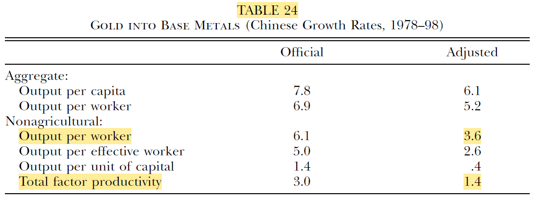
Aside: in this paper Young switches from the traditional growth accounting method (used in eg Young 1995) to the adjusted (“Harrodian”) method I described – which properly attributes the growth caused by capital accumulation induced by higher TFP, to TFP
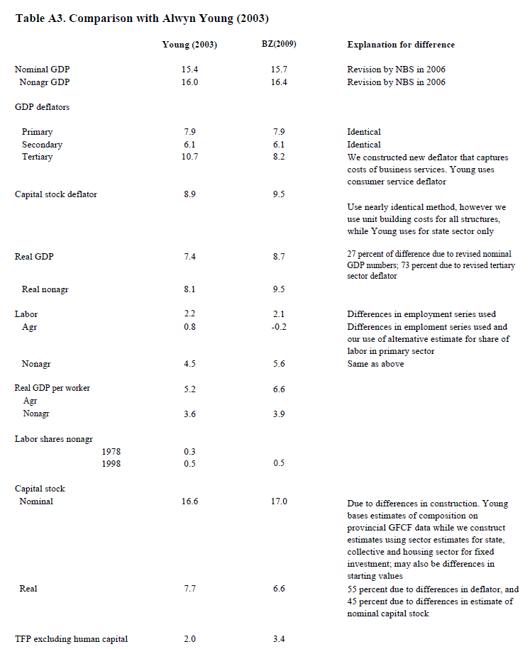
Brandt and Zhu (2010) revise Young’s estimate even further up – with updated data and correcting the deflator. Zhu (2012, JEP) is a very readable summary, showing:
From 1978-2007, TFP growth averaged 3.2% per year (!!) – again accounting for more 3/4 of GDPpc growth
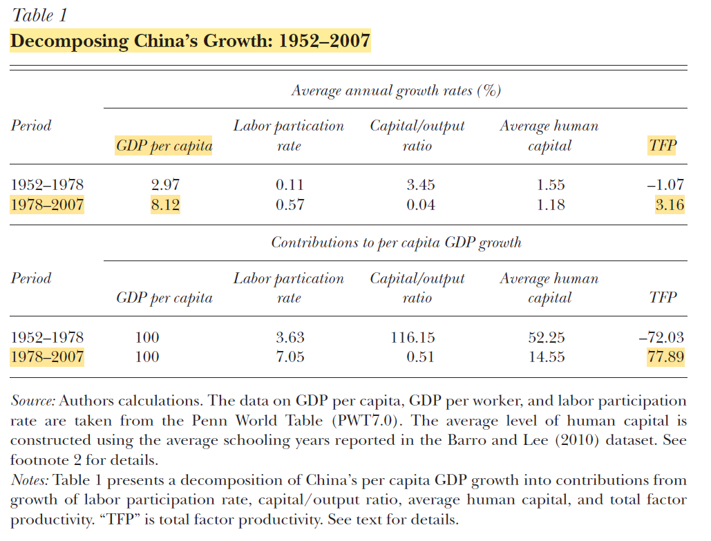
You can also see in that^ table an accounting for growth under Mao, 1952-1978: 3% growth in GDP per capita [on avg 💀], entirely due to K+H accumulation – annual TFP growth was -1%!!
If I had to recommend one paper here, it would be this Zhu (2010) paper
Will also note – Cheremukhin, Golosov, Guriev, and Tsyvinski (2015, 2024) do an interesting wedge accounting of the Chinese economy, mostly discussing pre-reform but also briefly post-reform. I’m not sure if their results match the rest of this thread

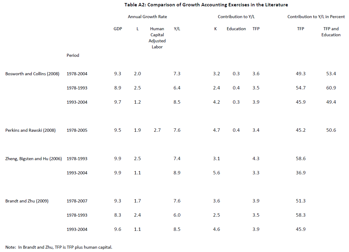
Other growth accounting papers covering the period up to 2008 also show 50-75% of Chinese growth is accounted for by TFP growth (Bosworth and Collins 2008; Zheng, Bigsten, and Hu 2009; Rajah and Leng (2022))
Ok, well that was part 1: TFP growth in China was high 1978-2007, accounting for 75% of Chinese growth over the period (after being quite negative under Mao)
Part 2 is: TFP growth has slowed down, a lot, since 2008 and the Great Recession
I haven’t been able to find any fantastic papers doing a growth accounting for the last decade (please send!!) and have been unwilling to wade into the data myself beyond the offensively crude cut I did here

BUT all the available evidence points to a major slowdown in Chinese TFP growth since 2008:
Brandt et al (2020) estimates a pre-2008 ten-year annual TFP growth of 2.8%
vs.
Post-2008 ten-year annual TFP growth of 0.7%
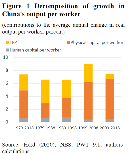
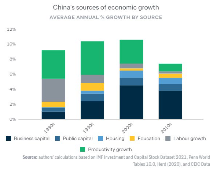
Rajah and Leng (2022) do a classic growth accounting decomposition, and also find TFP growth slowing substantially in the 2010s
Plausibly this slowdown is due in part to distortions caused by the policies enacted to avoid the global Great Recession?

Again, I would love to read more analysis of the Chinese TFP slowdown of the last 15 years / the Xi Jinping economy, please send links 😀
Ok, so:
1. Part 1 was that Chinese TFP growth was high after the reform & opening up
2. Part 2 was that TFP growth slowed substantially post-2008
What’s the future of Chinese growth?
The fundamental fact is that Chinese TFP is still far below that of the US: there is a lot of room left to run. China could still grow a lot. Obviously, the question is: will it?
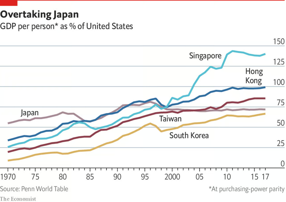
Zhu (2012) points out: in the ˜30 years post reform and opening up, China went from 3% of US TFP to 13% (in 2007)
In comparison:
Japan TFP 1950: 56% of US -> 83%
Korea TFP 1965: 43% of US -> 63%
Taiwan TFP 1950: 50% of US -> 80%
Again: China has a lot of room left to run...
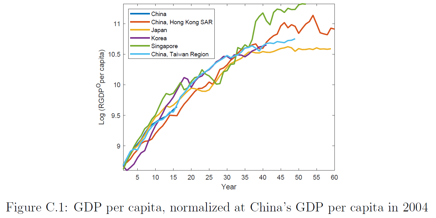
Here’s my quick and liable-to-be-incorrect figure showing “Chinese productivity has a lot of room left to grow”:
Plotting the Y/L trajectory for major East Asian economies vs. TFP – data simply pulled from PWT. Chinese TFP is low
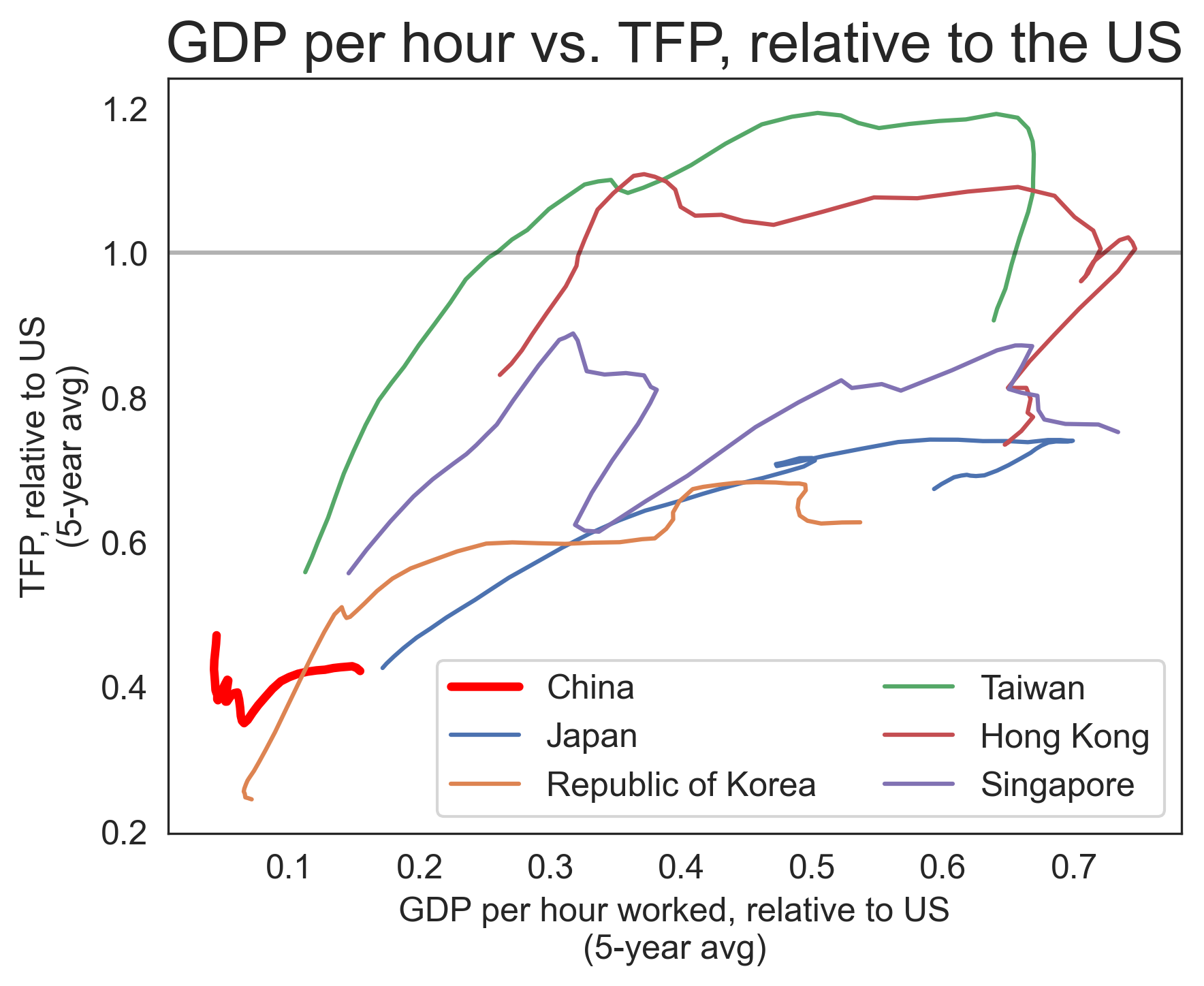
(That same PWT data, though, also shows Chinese TFP being flat relative to the US over the last 60 years, which contradicts the main thesis of this thread, so...
¯\_(ツ)_/¯)
(I would assume the PWT TFP estimate quality <<< the quality of the cited papers)
Anyway –
The best analysis that I could find on projecting future Chinese growth [modulo the singularity etc] is Rajah and Leng (2022), which uses a neoclassical framework
Rajah and Leng (2022) assume a continued gradual reduction in Chinese TFP growth until convergence to frontier TFP growth rates
Between a TFP slowdown, an aging population, and declining {urban population, housing, public investment} growth –
They forecast 3% GDP growth by 2030

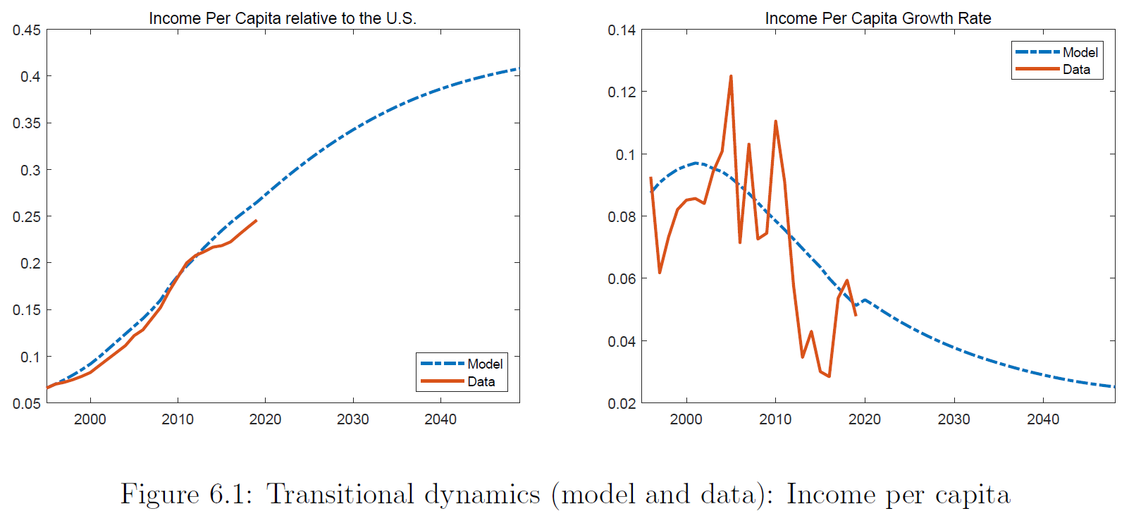
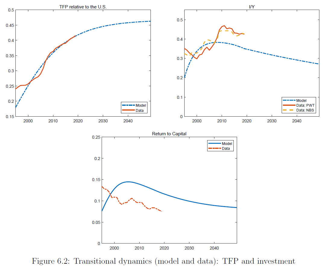
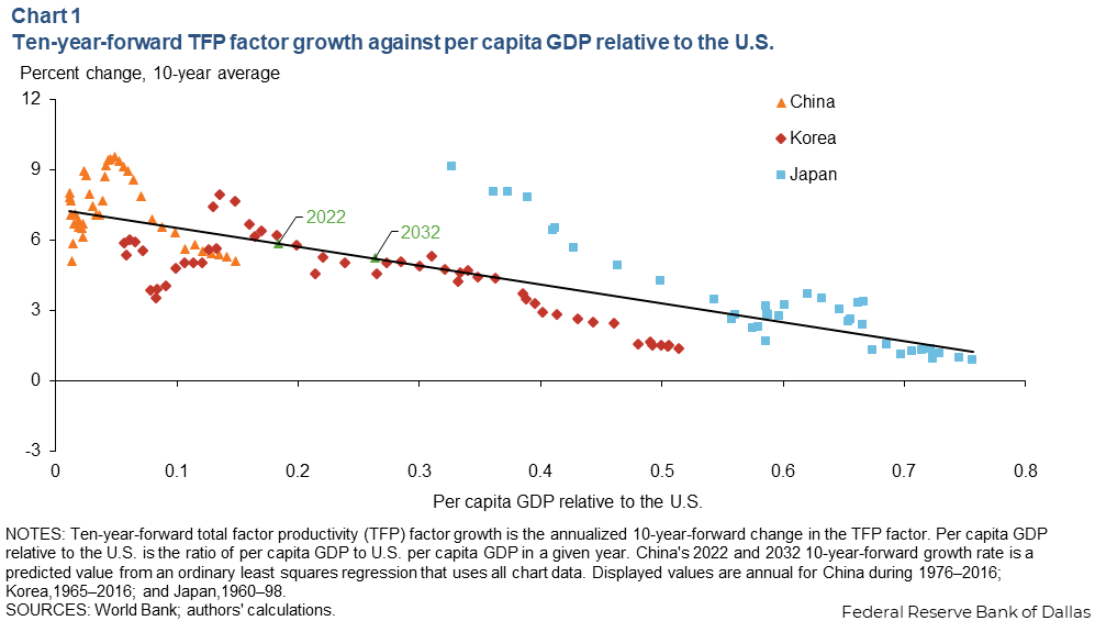
An even more direct approach to projecting future Chinese growth is Fernandez-Villaverde, Ohanian, and Yao (2023), where TFP growth is projected statistically
The idea is: China’s growth path has followed shockingly closely to other East Asian miracles. What if that continues:
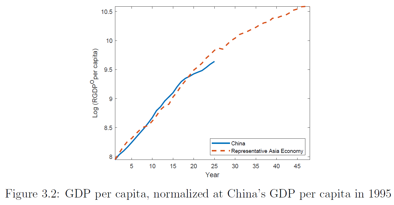
Again, additional references/corrections welcome
These threads brought to you by some binge reading before a big trip to China last month. Cold War II sucks but at least we’ve still got growth accounting 👍So that’s my read of the China growth accounting lit:
1. TFP growth was fast + was an important part of the miraculous decades of growth, which rejects crude Solow-ism
2. TFP growth has slowed down since 2008
3. There is a lot of room left that the PRC could run
Some bonus China economy charts from my lit binge:
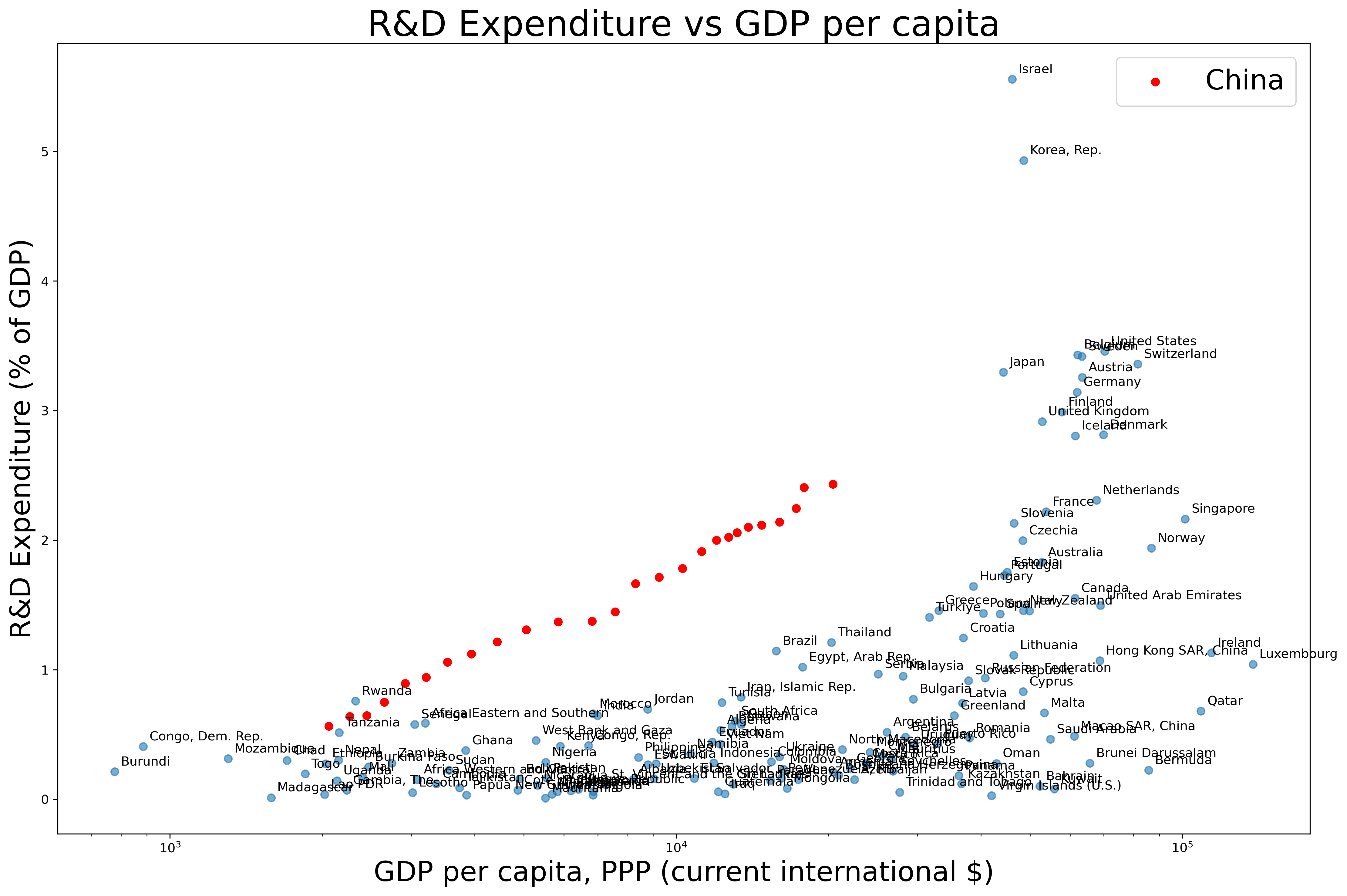
1) China is spending more on R&D than you would expect based on GDP per capita
(my update of a chart from Wei, Xie, and Zhang 2017)
2) Consensus long-term China real GDP growth forecasts:

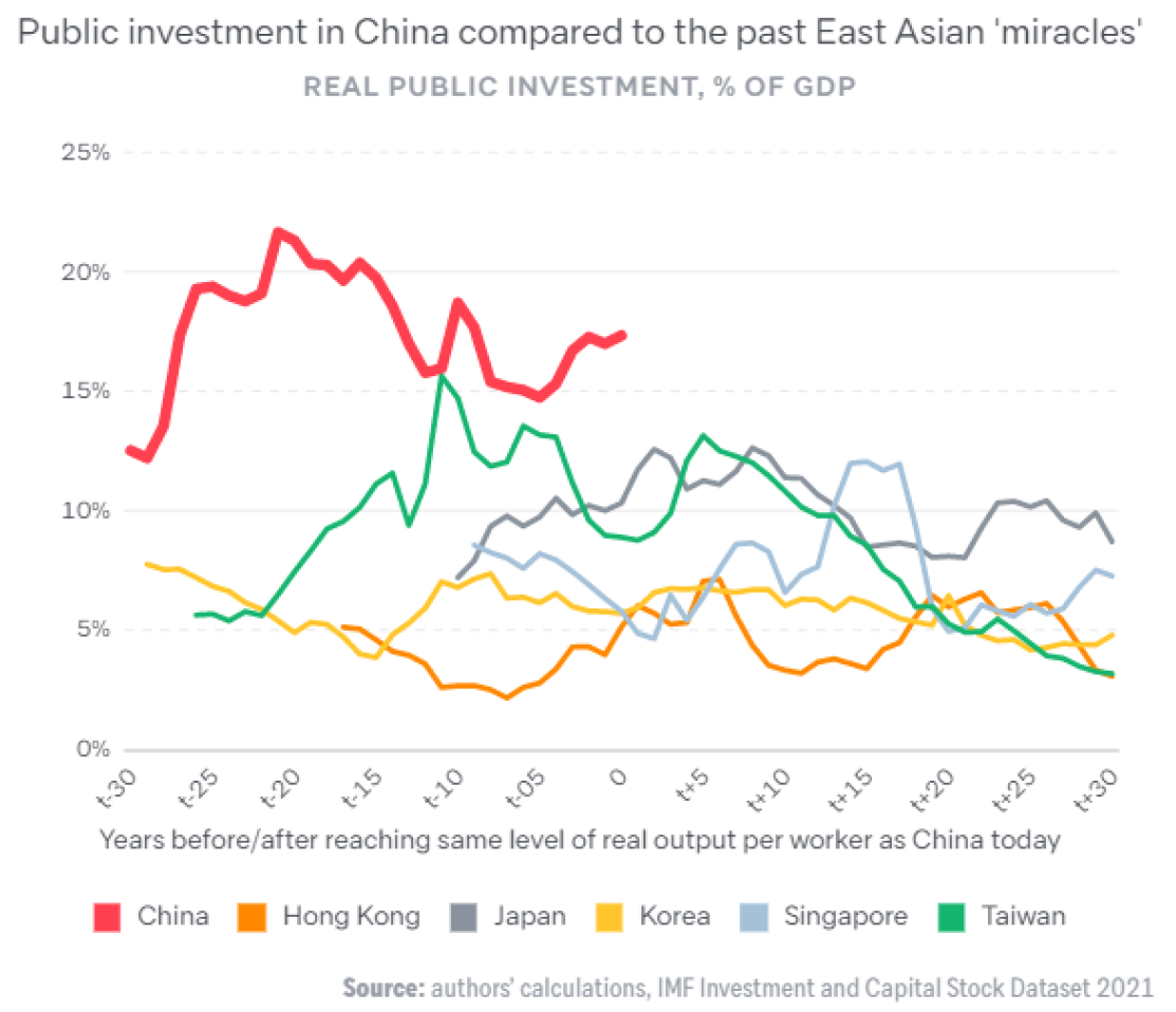
3) Chinese public investment has been higher than other East Asian miracles over the whole development trajectory (Rajah and Leng 2022):
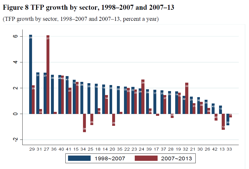
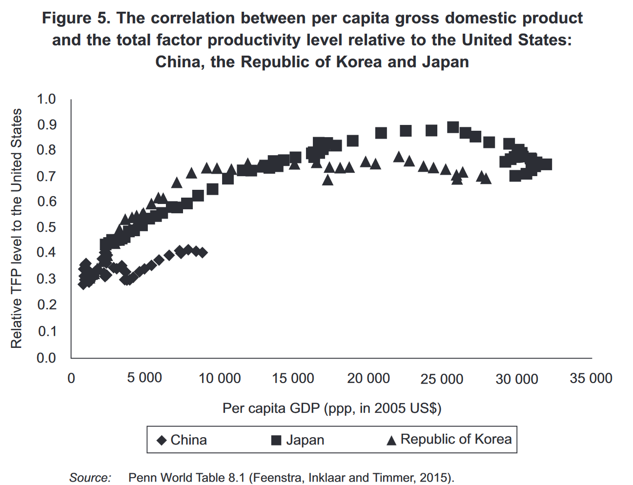
4) I haven’t looked closely into these TFP charts but they are interesting and plausibly more accurate than my similar quick and dirty one: (source 1, source 2
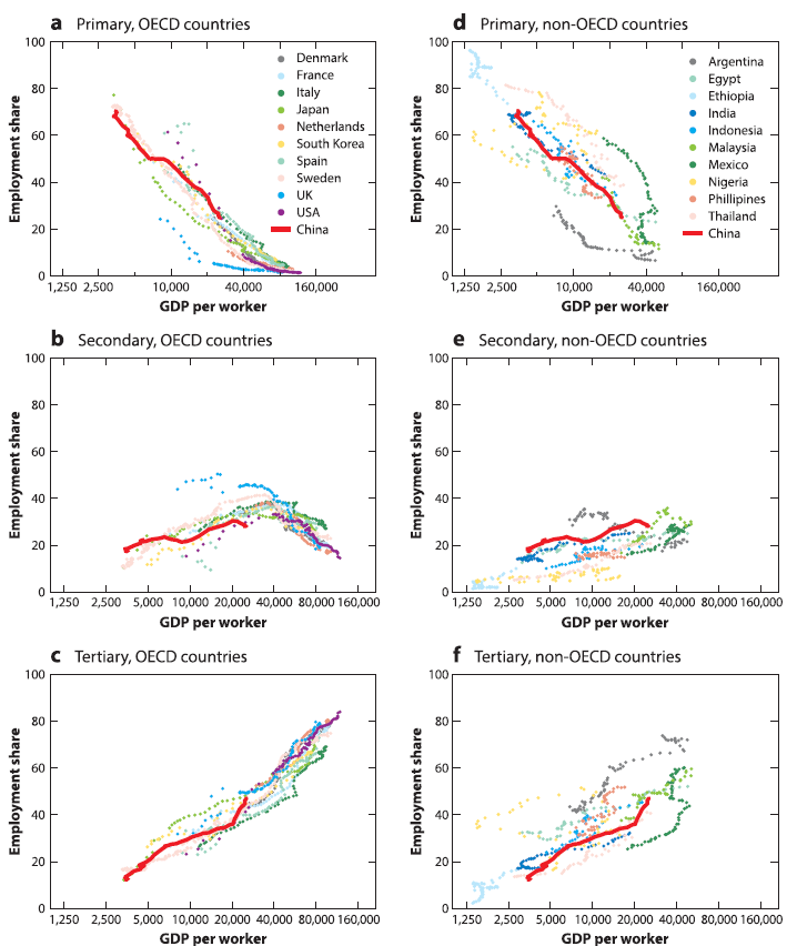
5) The Chinese economy is shifting towards services; and this trajectory is surprisingly predictable across countries (Chen, Pei, Song, and Zilibotti 2023)
[primary = agriculture; secondary = manufacturing; tertiary = services]
Bonus book recommendation: Yasheng Huang
Will hopefully do a thread on this but Yasheng Huang’s EAST is probably the best big think book on China I’ve read + great “applied political economy theory”
— Basil Halperin (@BasilHalperin) June 2, 2024
Bonus podcast recommendation: Yasheng Huang interview
Originally posted as a Twitter thread.
I think the Solow/neoclassical model is overrated *for explaining catch-up growth and convergence*
Some thoughts, as a prelude to a thread on Chinese growth accounting:
Let me frame the argument against Solow by appealing to the debate over the rapid growth of East Asian Tigers (Hong Kong, Singapore, South Korea, Taiwan) from 1960-2000:
1. Did the E. Asian Tigers grow fast because of rapid productivity improvement?
vs.
2. Was it merely Solow catch-up growth: poor countries start off with few machines...
...build more (“capital accumulation”)...
...and grow faster until they have enough machines (“convergence”)
Alwyn Young (1992, 1995) famously argued that the rapid growth of the East Asian Tigers was largely not due to productivity growth
Paul Krugman popularized this view in an influential Foreign Affairs article, “The Myth of Asia’s Miracle”, suggesting effectively zero TFP growth
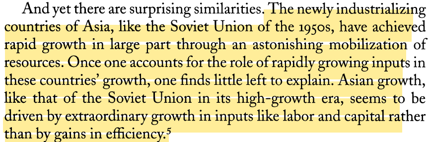
From Young’s legendarily careful data work, it was argued Tiger growth was merely capital accumulation: Solow-style catch up growth
The growth accounting from Young (1995) – “the tyranny of numbers” – shows TFP growth explaining at most 30% of Tiger growth
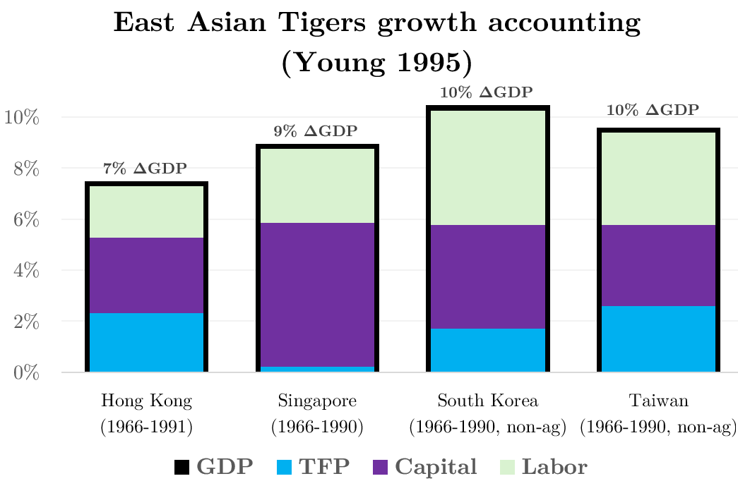
That is: Hong Kong, Taiwan, S Korea, and especially Singapore simply started in 1960 with few machines and low education
The rapid growth merely came from building more machines and shuttling more kids through school – not from producing things more intelligently (TFP growth)
This Krugman-Young story is precisely the simple story of convergence of Solow!
Again: poor countries start off with few machines, then build more (“capital accumulation”) and so grow faster until they have enough machines (“convergence”)
This is the view of the E. Asian Tiger experience I had accepted, until recently
There are a few issues, with the overriding fact being that: growth accounting is actually just really hard. Empirically tough, but also conceptually
I’ll focus on a conceptual issue (“wonkish”)
Higher TFP causes capital accumulation:
If you get more productive, you want to (gradually) build more machines
=> AND those machines cause more growth
Should we attribute that higher growth to the machines, or to the productivity?
Traditional growth accounting gives credit for growth caused by that extra capital to capital itself
But it really makes more sense to give (long-run) credit to the higher productivity, which is itself causing the extra capital!
Brief Cobb-Douglas math for the curious (in logs):
Traditional growth accounting: Y = A + α⋅K + (1-α)⋅L
Instead: Y – L = (1/(1- α))⋅A + (α/(1-α))⋅(K – Y)
(See eg Klenow-Rodriguez-Clare 1997, or Jones 2016 sec 2.1)
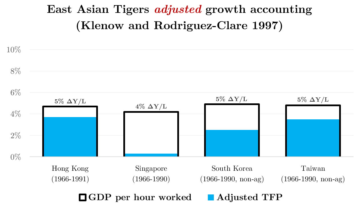
So for example, Klenow and Rodriguez-Clare (1997) reanalyze the East Asian Tiger experience: properly accounting for TFP-induced capital accumulation + analyzing Y/L rather than Y
They find that TFP growth accounts for 50-75% of Tiger growth (!), except for Singapore
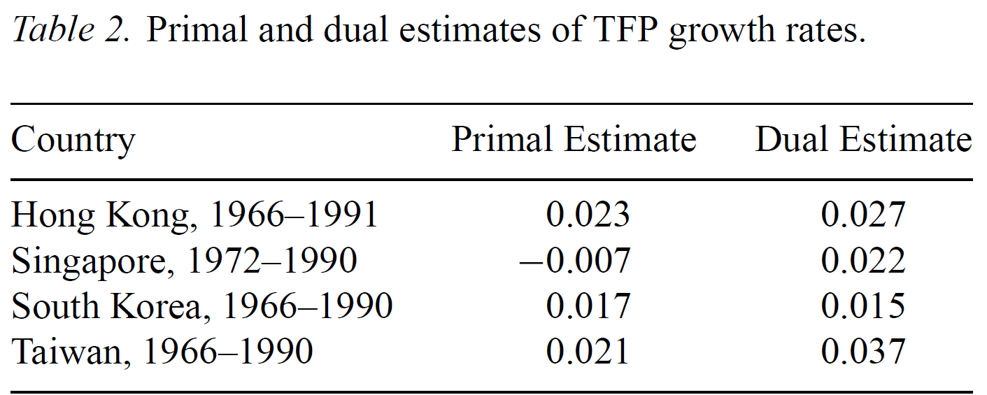
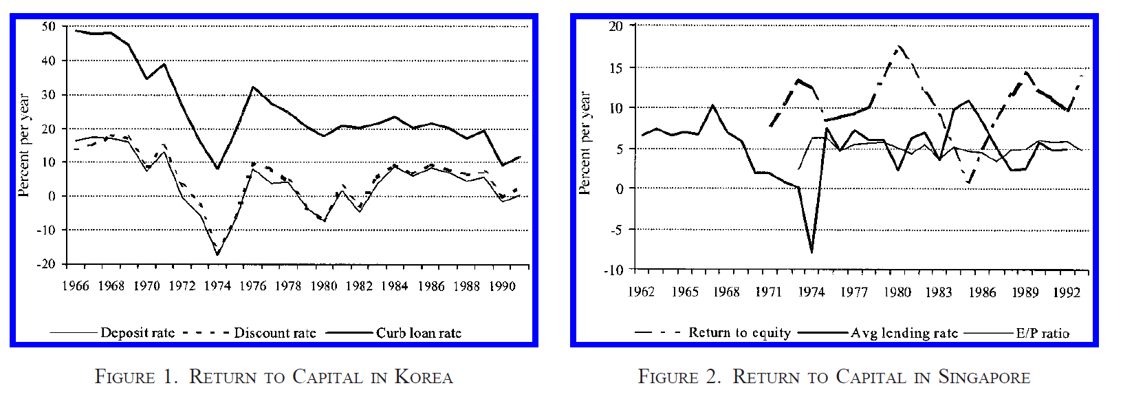
Briefly, another critique of the neoclassical (Young/Krugman) view is Hsieh (2002), who argues that the rate of return on capital didn’t fall in Singapore, as the neoclassical/Solow model would predict – implying higher TFP growth. This is the “dual approach” to growth accounting
[PART 2: an alternative view of catch-up growth]
Just from armchair theorizing, the Solow model view that faster catch-up growth is all due to capital accumulation feels a little odd, IMO
Do poor countries really grow fast because they’re just accumulating capital (building more machines, etc), a la Solow? Isn’t that kind of crazy?
A priori, aren’t poor countries also catching up by **importing technology**?
IMO the Solow model is plausibly... overrated 😎
Overrated, since Solow attributes fast catch-up growth entirely to temporarily high capital accumulation – and not at all to higher technological growth
Poor countries also have low productivity! Shouldn’t some of the catch-up growth come from simply imitating tech leaders?
(that^ tweet is the punchline of the thread!)
The first attempt (AFAIK) to model catch-up growth as being caused by technological diffusion, rather than Solow-style capital accumulation, was Barro and Sala-i-Martin (1997). The Acemoglu textbook ch. 18 also has a clear exposition
These models do what you would expect:
“Imitation is cheaper than invention”, so countries behind the frontier can copy ideas cheaply and grow TFP and GDP quickly
As they catch up in terms of TFP, it gets more expensive to copy ideas – you’re trying to imitate semiconductors instead of tractors – and growth falls
In the long run, all countries grow at the rate of the frontier – and the frontier is nicely determined exactly as in the canonical growth models
The framework matches the armchair view of historical catch-up growth – it is driven in part by poor countries getting more productive by copying technology
That said, obviously a lot of catch-up growth is ALSO surely due to Solow-style capital accumulation
A crude extrapolation is 50-50 on average: half productivity catch-up + half capital accumulation catch-up
I haven’t seen a paper doing the decomposition across all catch-up growth episodes (many papers look at all countries/times – mixing in BGP level differences, I think)
Maybe postwar Europe (which surely motivated Solow) – with the rebuilding after the destruction – was catch-up growth driven mostly by capital accumulation, not technology diffusion
(Though maybe not, based on this dirty cut adapted from Dietz Vollrath?)
Recent Vollrath blog seems to show that
— Basil Halperin (@BasilHalperin) March 26, 2023
Postwar European rapid growth was not catch-up growth -- i.e. it wasn't Solow-style capital (re)accumulation -- which I thought was the consensus view
It was TFP growth (?)https://t.co/HsZe9RaEmA pic.twitter.com/e7N6DnVD1o
Convergence is, obviously, a huge topic in the lit and I feel like there must have been more study of this / someone else must have framed the question this way:
“Is catch-up growth due to Solow-style capital accumulation vs. technology diffusion?”
References very welcome!
Originally posted as a Twitter thread.
Miscellaneous things I learned in [econ] grad school:
1. The returns to experience are high(er than I thought)
- Someone who has studied a single topic for a decade or two or three really does know a LOT about that topic
One way you can see this: the way experienced faculty have seemingly photographic memories of subsections of papers and interactions in seminars from years ago --
In the same way that experienced NBA/chess players can have photographic memories of games
2. Even in the 6-year PhD, you can see slow-growing returns to experience. This feels weird!
Eg only after years of seminars did I begin to feel attending was ever worth the time (compared to just reading the paper). The brain sometimes needs LOTS of training data to rewire
3. All that said though, youth/fresh eyes are still crazy powerful for "thinking about things" ie research
- It's bonkers that a 20-year-old can bring insight to a topic studied for ***decades*** by others
4. It's hard to keep learning new things while doing research
While doing research, it feels like there is a temptation to just grind on the research, and not continually invest in learning new things. Tough balance 🙃
The pressure is to *produce now*, which can lead to myopic underinvestment in human capital
"Fail[ing] to continue to plant the little acorns from which the mighty oak trees grow", as Hamming put it. Extremely real!
On the experience of grad school:
5. It's more like high school than undergrad: it's a smaller environment, everyone knows each other for years; it can feel like you're less in control of your fate (imho)
6. Or: grad school is more like being unemployed than it is like being employed. The amount of free time is nuts and it drives people mad
Unstructured time can really screw with people's heads. In that respect, grad school is more like unemployment than high school for a lot of people.
— Cameron Harwick 👾🏛 (@C_Harwick) October 28, 2020
7. Academia in general has fractal complexity (this is true of many careers of course): in a lot of ways, the more you learn about what it's like, the more you realize you don't know
(🙃)
8. For example -- this was embarrassingly not clear to me before starting the PhD; trigger warning: naivete -- the classes are 90%+ about teching up, not about discussion
Or:
9. At the frontier, it is not clear whether (written) papers or (oral) seminars matter more...
From the outside, you only see the papers -- it looks like academia consists of the papers. On the inside, it's clear there's less reading and the seminars matter a lot
10. In general, academia/grad school is an oral culture (i.e., not a written culture), and it pays to just talk with people to share information
You can overinvest, but taking the break from research to get coffee with friends and just blab has high EV, in my experience
11. Relatedly: everyone warns you about spending too much time being overly strategic ("just work on your research")
But you can also easily be not-strategic-enough! You see people on both sides of the Laffer peak
12. Sometimes I think of academia as a royal court:
- clear hierarchy
- reputation/status are omnipresent
- *everyone knows everyone* (not really, but it can feel like it), literal *names* matter a lot
- obviously the exclusivity
- ceremony, patronage, etiquette, court intrigue..
^"being like a royal court" has both negative but definitely also positive aspects, to be clear!
cf
Academia has an "honor" culture similar to US South
— Arpit Gupta (@arpitrage) July 9, 2019
In the South, politeness rested on undercurrent of violence against threats to honor
Academia: delicate balance of power from implicit threats of negative referee reports, discussions, tenure letters etcsustains niceness
13. Something that took me longer to learn than I'd like to admit --
Papers are mini textbooks. It's not about having "one big insight" (maybe it used to be). It's about fleshing out *everything* related to your topic (within some bounds)
14. On fields. We're still living in the aftermath of the credibility revolution
- We're still picking the low-hanging empirical fruit made available thanks to these tools; and status in the profession is allocated accordingly
plausibly this is efficient ¯\_(ツ)_/¯
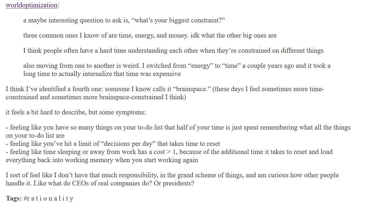
15. On conferences. Conferences (for me at least) have to be exercises in ruthless energy management
16. Relatedly, for doing theory research: it was weird switching from my entire previous life where "time" was the biggest constraint to "energy" being the biggest constraint
(though for most empirical/coding work it's still "time" in my experience)
17. In education, *teaching effort* is that which is scarce
As a student, I would hear education policy recommendation X and think it sounds sensible. As a teacher, I hear X and think about "well that has a benefit, ...but it requires costly effort from the teacher"
18. (A few) things I still want to understand:
(i) The division of labor in different kinds of academic teams. Team production functions vary a lot?
(ii) The life cycle of the academic researcher. How sharply do goals change over time? How much of that is constrained vs. not?
Joint with Trevor Chow and J. Zachary Mazlish. Also posted at the EA Forum. November 2023 update: This post is now an academic paper, here, with some different emphasis and some new empirical evidence
In this post, we point out that short AI timelines would cause real interest rates to be high, and would do so under expectations of either unaligned or aligned AI. However, 30- to 50-year real interest rates are low. We argue that this suggests one of two possibilities:
In the rest of this post we flesh out this argument.
An order-of-magnitude estimate is that, if markets are getting this wrong, then there is easily $1 trillion lying on the table in the US treasury bond market alone – setting aside the enormous implications for every other asset class.
Interpretation. We view our argument as the best existing outside view evidence on AI timelines – but also as only one model among a mixture of models that you should consider when thinking about AI timelines. The logic here is a simple implication of a few basic concepts in orthodox economic theory and some supporting empirical evidence, which is important because the unprecedented nature of transformative AI makes “reference class”-based outside views difficult to construct. This outside view approach contrasts with, and complements, an inside view approach, which attempts to build a detailed structural model of the world to forecast timelines (e.g. Cotra 2020; see also Nostalgebraist 2022).
Outline. If you want a short version of the argument, sections I and II (700 words) are the heart of the post. Additionally, the section titles are themselves summaries, and we use text formatting to highlight key ideas.
Real interest rates reflect, among other things:
This claim is compactly summarized in the “Ramsey rule” (and the only math that we will introduce in this post), a version of the “Euler equation” that in one form or another lies at the heart of every theory and model of dynamic macroeconomics:
r = ρ + σg
where:
(Internalizing the meaning of these Greek letters is wholly not necessary.)
While more elaborate macroeconomic theories vary this equation in interesting and important ways, it is common to all of these theories that the real interest rate is higher when either (1) the time discount rate is high or (2) future growth is expected to be high.
We now provide some intuition for these claims.
Time discounting and mortality risk. Time discounting refers to how much people discount the future relative to the present, which captures both (i) intrinsic preference for the present relative to the future and (ii) the probability of death.
The intuition for why the probability of death raises the real rate is the following. Suppose we expect with high probability that humanity will go extinct next year. Then there is no reason to save today: no one will be around to use the savings. This pushes up the real interest rate, since there is less money available for lending.
Economic growth. To understand why higher economic growth raises the real interest rate, the intuition is similar. If we expect to be wildly rich next year, then there is also no reason to save today: we are going to be tremendously rich, so we might as well use our money today while we’re still comparatively poor.
(For the formal math of the Euler equation, Baker, Delong, and Krugman 2005 is a useful reference. The core intuition is that either mortality risk or the prospect of utopian abundance reduces the supply of savings, due to consumption smoothing logic, which pushes up real interest rates.)
Transformative AI and real rates. Transformative AI would either raise the risk of extinction (if unaligned), or raise economic growth rates (if aligned).
Therefore, based on the economic logic above, the prospect of transformative AI – unaligned or aligned – will result in high real interest rates. This is the key claim of this post.
As an example in the aligned case, Davidson (2021) usefully defines AI-induced “explosive growth” as an increase in growth rates to at least 30% annually. Under a baseline calibration where σ=1 and ρ=0.01, and importantly assuming growth rates are known with certainty, the Euler equation implies that moving from 2% growth to 30% growth would raise real rates from 3% to 31%!
For comparison, real rates in the data we discuss below have never gone above 5%.
(In using terms like “transformative AI” or “advanced AI”, we refer to the cluster of concepts discussed in Yudkowsky 2008, Bostrom 2014, Cotra 2020, Carlsmith 2021, Davidson 2021, Karnofsky 2022, and related literature: AI technology that precipitates a transition comparable to the agricultural or industrial revolutions.)
The US 30-year real interest rate ended 2022 at 1.6%. Over the full year it averaged 0.7%, and as recently as March was below zero. Looking at a shorter time horizon, the US 10-year real interest rate is 1.6%, and similarly was below negative one percent as recently as March.

(Data sources used here are explained in section V.)
The UK in autumn 2021 sold a 50-year real bond with a -2.4% rate at the time. Real rates on analogous bonds in other developed countries in recent years have been similarly low/negative for the longest horizons available. Austria has a 100-year nominal bond – being nominal should make its rate higher due to expected inflation – with yields less than 3%.
Thus the conclusion previewed above: financial markets, as evidenced by real interest rates, are not expecting a high probability of either AI-induced growth acceleration or elevated existential risk, on at least a 30-50 year time horizon.
In this section we briefly consider some potentially important complications.
Uncertainty. The Euler equation and the intuition described above assumed certainty about AI timelines, but taking into account uncertainty does not change the core logic. With uncertainty about the future economic growth rate, then the real interest rate reflects the expected future economic growth rate, where importantly the expectation is taken over the risk-neutral measure: in brief, probabilities of different states are reweighted by their marginal utility. We return to this in our quantitative model below.
Takeoff speeds. Nothing in the logic above relating growth to real rates depends on slow vs. fast takeoff speed; the argument can be reread under either assumption and nothing changes. Likewise, when considering the case of aligned AI, rates should be elevated whether economic growth starts to rise more rapidly before advanced AI is developed or only does so afterwards. What matters is that GDP – or really, consumption – ends up high within the time horizon under consideration. As long as future consumption will be high within the time horizon, then there is less motive to save today (“consumption smoothing”), pushing up the real rate.
Inequality. The logic above assumed that the development of transformative AI affects everyone equally. This is a reasonable assumption in the case of unaligned AI, where it is thought that all of humanity will be evaporated. However, when considering aligned AI, it may be thought that only some will benefit, and therefore real interest rates will not move much: if only an elite Silicon Valley minority is expected to have utopian wealth next year, then everyone else may very well still choose to save today.
It is indeed the case that inequality in expected gains from transformative AI would dampen the impact on real rates, but this argument should not be overrated. First, asset prices can be crudely thought of as reflecting a wealth-weighted average across investors. Even if only an elite minority becomes fabulously wealthy, it is their desire for consumption smoothing which will end up dominating the determination of the real rate. Second, truly transformative AI leading to 30%+ economy-wide growth (“Moore’s law for everything”) would not be possible without having economy-wide benefits.
Stocks. One naive objection to the argument here would be the claim that real interest rates sound like an odd, arbitrary asset price to consider; certainly stock prices are the asset price that receive the most media attention.
In appendix 1, we explain that the level of the real interest rate affects every asset price: stocks for instance reflect the present discounted value of future dividends; and real interest rates determine the discount rate used to discount those future dividends. Thus, if real interest rates are ‘wrong’, every asset price is wrong. If real interest rates are wrong, a lot of money is on the table, a point to which we return in section X.
We also argue that stock prices in particular are not a useful indicator of market expectations of AI timelines. Above all, high stock prices of chipmakers or companies like Alphabet (parent of DeepMind) could only reflect expectations for aligned AI and could not be informative of the risk of unaligned AI. Additionally, as we explain further in the appendix, aligned AI could even lower equity prices, by pushing up discount rates.
In section I, we gave theoretical intuition for why higher expected growth or higher existential risk would result in higher interest rates: expectations for such high growth or mortality risk would lead people to want to save less and borrow more today. In this section and the next two, we showcase some simple empirical evidence that the predicted relationships hold in the available data.
Measuring real rates. To compare historical real interest rates to historical growth, we need to measure real interest rates.
Most bonds historically have been nominal, where the yield is not adjusted for changes in inflation. Therefore, the vast majority of research studying real interest rates starts with nominal interest rates, attempts to construct an estimate of expected inflation using some statistical model, and then subtracts this estimate of expected inflation from the nominal rate to get an estimated real interest rate. However, constructing measures of inflation expectations is extremely difficult, and as a result most papers in this literature are not very informative.
Additionally, most bonds historically have had some risk of default. Adjusting for this default premium is also extremely difficult, which in particular complicates analysis of long-run interest rate trends.
The difficulty in measuring real rates is one of the main causes, in our view, of Tyler Cowen’s Third Law: “all propositions about real interest rates are wrong”. Throughout this piece, we are badly violating this (Godelian) Third Law. In appendix 2, we expand on our argument that the source of Tyler’s Third Law is measurement issues in the extant literature, together with some separate, frequent conceptual errors.
Our approach. We take a more direct approach.
Real rates. For our primary analysis, we instead use market real interest rates from inflation-linked bonds. Because we use interest rates directly from inflation-linked bonds – instead of constructing shoddy estimates of inflation expectations to use with nominal interest rates – this approach avoids the measurement issue just discussed (and, we argue, allows us to escape Cowen’s Third Law).
To our knowledge, prior literature has not used real rates from inflation-linked bonds only because these bonds are comparatively new. Using inflation-linked bonds confines our sample to the last ∼20 years in the US, the last ∼30 in the UK/Australia/Canada. Before that, inflation-linked bonds didn’t exist. Other countries have data for even fewer years and less liquid bond markets.
(The yields on inflation-linked bonds are not perfect measures of real rates, because of risk premia, liquidity issues, and some subtle issues with the way these securities are structured. You can build a model and attempt to strip out these issues; here, we will just use the raw rates. If you prefer to think of these empirics as “are inflation-linked bond yields predictive of future real growth” rather than “are real rates predictive of future real growth”, that interpretation is still sufficient for the logic of this post.)
Nominal rates. Because there are only 20 or 30 years of data on real interest rates from inflation-linked bonds, we supplement our data by also considering unadjusted nominal interest rates. Nominal interest rates reflect real interest rates plus inflation expectations, so it is not appropriate to compare nominal interest rates to real GDP growth.
Instead, analogously to comparing real interest rates to real GDP growth, we compare nominal interest rates to nominal GDP growth. The latter is not an ideal comparison under economic theory – and inflation variability could swamp real growth variability – but we argue that this approach is simple and transparent.
Looking at nominal rates allows us to have a very large sample of countries for many decades: we use OECD data on nominal rates available for up to 70 years across 39 countries.
The goal of this section is to show that real interest rates have correlated with future real economic growth, and secondarily, that nominal interest rates have correlated with future nominal economic growth. We also briefly discuss the state of empirical evidence on the correlation between real rates and existential risk.
Real rates vs. real growth. A first cut at the data suggests that, indeed, higher real rates today predict higher real growth in the future:

To see how to read these graphs, take the left-most graph (“10-year horizon”) for example. The x-axis shows the level of the real interest rate, as reflected on 10-year inflation linked bonds. The y-axis shows average real GDP growth over the following 10 years.
The middle and right hand graphs show the same, at the 15-year and 20-year horizons. The scatter plot shows all available data for the US (since 1999), the UK (since 1985), Australia (since 1995), and Canada (since 1991). (Data for Australia and Canada is only available at the 10-year horizon, and comes from Augur Labs.)
Eyeballing the figure, there appears to be a strong relationship between real interest rates today and future economic growth over the next 10-20 years.
To our knowledge, this simple stylized fact is novel.
Caveats. “Eyeballing it” is not a formal econometric method; but, this is a blog post not a journal article (TIABPNAJA). We do not perform any formal statistical tests here, but we do want to acknowledge some important statistical points and other caveats.
First, the data points in the scatter plot are not statistically independent: real rates and growth are both persistent variables; the data points contain overlapping periods; and growth rates in these four countries are correlated. These issues are evident even from eyeballing the time series. Second, of course this relationship is not causally identified: we do not have exogenous variation in real growth rates. (If you have ideas for identifying the causal effect of higher real growth expectations on real rates, we would love to discuss with you.)
Relatedly, many other things are changing in the world which are likely to affect real rates. Population growth is slowing, retirement is lengthening, the population is aging. But under AI-driven “explosive” growth – again say 30%+ annual growth, following the excellent analysis of Davidson (2021) – then, we might reasonably expect that this massive of an increase in the growth rate would drown out the impact of any other factors.
Nominal rates vs. nominal growth. Turning now to evidence from nominal interest rates, recall that the usefulness of this exercise is that while there only exists 20 or 30 years of data on real interest rates for two countries, there is much more data on nominal interest rates.
We simply take all available data on 10-year nominal rates from the set of 39 OECD countries since 1954. The following scatterplot compares the 10-year nominal interest versus nominal GDP growth over the succeeding ten years by country:

Again, there is a strong positive – if certainly not perfect – relationship. (For example, the outlier brown dots at the bottom of the graph are Greece, whose high interest rates despite negative NGDP growth reflect high default risk during an economic depression.)
The same set of nontrivial caveats apply to this analysis as above.
We consider this data from nominal rates to be significantly weaker evidence than the evidence from real rates, but corroboration nonetheless.
Backing out market-implied timelines. Taking the univariate pooled OLS results from the real rate data far too seriously, the fact that the 10-year real rate in the US ended 2022 at 1.6% would predict average annual real GDP growth of 2.6% over the next 10 years in the US; the analogous interest rate of -0.2% in the UK would predict 0.7% annual growth over the next 10 years in the UK. Such growth rates, clearly, are not compatible with the arrival of transformative aligned AI within this horizon.
We have argued that in the theory, real rates should be higher in the face of high economic growth or high mortality risk; empirically, so far, we have only shown a relationship between real rates and growth, but not between real rates and mortality.
Showing that real rates accurately reflect changes in existential risk is very difficult, because there is no word-of-god measurement of how existential risk has evolved over time.
We would be very interested in pursuing new empirical research examining “asset pricing under existential risk”. In appendix 3, we perform a scorched-earth literature review and find essentially zero existing empirical evidence on real rates and existential risks.
Disaster risk. In particular, the extant literature does not study existential risks but instead “merely” disaster risks, under which real assets are devastated but humanity is not exterminated. Disaster risks do not necessarily raise real rates – indeed, such risks are thought to lower real rates due to precautionary savings. That notwithstanding, some highlights of the appendix review include a small set of papers finding that individuals with a higher perceived risk of nuclear conflict during the Cold War saved less, as well as a paper noting that equities which were headquartered in cities more likely to be targeted by Soviet missiles did worse during the Cuban missile crisis (see also). Our assessment is that these and the other available papers on disaster risks discussed in the appendix have severe limitations for the purposes here.
Individual mortality risk. We judge that the best evidence on this topic comes instead from examining the relationship between individual mortality risk and savings/investment behavior. The logic we provided was that if humanity will be extinct next year, then there is no reason to save, pushing up the real rate. Similar logic says that at the individual level, a higher risk of death for any reason should lead to lower savings and less investment in human capital. Examples of lower savings at the individual level need not raise interest rates at the economy-wide level, but do provide evidence for the mechanism whereby extinction risk should lead to lower saving and thus higher interest rates.
One example comes from Malawi, where the provision of a new AIDS therapy caused a significant increase in life expectancy. Using spatial and temporal variation in where and when these therapeutics were rolled out, it was found that increased life expectancy results in more savings and more human capital investment in the form of education spending. Another experiment in Malawi provided information to correct pessimistic priors about life expectancy, and found that higher life expectancy directly caused more investment in agriculture and livestock.
A third example comes from testing for Huntington’s disease, a disease which causes a meaningful drop in life expectancy to around 60 years. Using variation in when people are diagnosed with Huntington’s, it has been found that those who learn they carry the gene for Huntington’s earlier are 30 percentage points less likely to finish college, which is a significant fall in their human capital investment.
Studying the effect on savings and real rates from increased life expectancy at the population level is potentially intractable, but would be interesting to consider further. Again, in our assessment, the best empirical evidence available right now comes from the research on individual “existential” risks and suggests that real rates should increase with existential risk.
Section VI used historical data to go from the current real rate to a very crude market-implied forecast of growth rates; in this section, we instead use a model to go from existing forecasts of AI timelines to timeline-implied real rates. We aim to show that under short AI timelines, real interest rates would be unrealistically elevated.
This is a useful exercise for three reasons. First, the historical data is only able to speak to growth forecasts, and therefore only able to provide a forecast under the possibly incorrect assumption of aligned AI. Second, the empirical forecast assumes a linear relationship between the real rate and growth, which may not be reasonable for a massive change caused by transformative AI. Third and quite important, the historical data cannot transparently tell us anything about uncertainty and the market’s beliefs about the full probability distribution of AI timelines.
We use the canonical (and nonlinear) version of the Euler equation – the model discussed in section I – but now allow for uncertainty on both how soon transformative AI will be developed and whether or not it will be aligned. The model takes as its key inputs (1) a probability of transformative AI each year, and (2) a probability that such technology is aligned.
The model is a simple application of the stochastic Euler equation under an isoelastic utility function. We use the following as a baseline, before considering alternative probabilities:
Thus, to summarize: by default, GDP grows at 1.8% per year. Every year, there is some probability (based on Cotra) that transformative AI is developed. If it is developed, there is a 15% probability the world ends, and an 85% chance GDP growth jumps to 30% per year.
We have built a spreadsheet here that allows you to tinker with the numbers yourself, such as adjusting the growth rate under aligned AI, to see what your timelines and probability of alignment would imply for the real interest rate. (It also contains the full Euler equation formula generating the results, for those who want the mathematical details.) We first estimate real rates under the baseline calibration above, before considering variations in the critical inputs.
Baseline results. The model predicts that under zero probability of transformative AI, the real rate at any horizon would be 2.8%. In comparison, under the baseline calibration just described based on Cotra timelines, the real rate at a 30-year horizon would be pushed up to 5.9% – roughly three percentage points higher.
For comparison, the 30-year real rate in the US is currently 1.6%.
While the simple Euler equation somewhat overpredicts the level of the real interest rate even under zero probability of transformative AI – the 2.8% in the model versus the 1.6% in the data – this overprediction is explainable by the radical simplicity of the model that we use and is a known issue in the literature. Adding other factors (e.g. precautionary savings) to the model would lower the level. Changing the level does not change its directional predictions, which help quantitatively explain the fall in real rates over the past ∼30 years.
Therefore, what is most informative is the three percentage point difference between the real rate under Cotra timelines (5.9%) versus under no prospect of transformative AI (2.8%): Cotra timelines imply real interest rates substantially higher than their current levels.
Now, from this baseline estimate, we can also consider varying the key inputs.
Varying assumptions on P(misaligned|AGI). First consider changing the assumption that advanced AI is 15% likely to be unaligned (conditional on the development of AGI). Varying this parameter does not have a large impact: moving from 0% to 100% probability of misalignment raises the model’s predicted real rate from 5.8% only to 6.3%.

Varying assumptions on timelines. Second, consider making timelines shorter or longer. In particular, consider varying the probability of development by 2043, which we use as a benchmark per the FTX Future Fund.
We scale the Cotra timelines up and down to vary the probability of development by 2043. (Specifically: we target a specific cumulative probability of development by 2043; and, following Cotra, if the annual probability up until 2030 is x, then it is 1.5x in the subsequent seven years up through 2036, and it is 2x in the remaining years of the 30-year window.)
As the next figure shows and as one might expect, shorter AI timelines have a very large impact on the model’s estimate for the real rate.

These results strongly suggest that any timeline shorter than or equal to the Cotra timeline is not being expected by financial markets.
While it is not possible to back out exact numbers for the market’s implicit forecast for AI timelines, it is reasonable to say that the market is decisively rejecting – i.e., putting very low probability on – the development of transformative AI in the very near term, say within the next ten years.
Consider the following examples of extremely short timelines:
Real rate movements of these magnitudes are wildly counterfactual. As previously noted, real rates in the data used above have never gone above even 5%.
Stagnation. As a robustness check, in the configurable spreadsheet we allow you to place some yearly probability on the economy stagnating and growing at 0% per year from thereon. Even with a 20% chance of stagnation by 2053 (higher than realistic), under Cotra timelines, the model generates a 2.1% increase in 30-year rates.
Recent market movements. Real rates have increased around two percentage points since the start of 2022, with the 30-year real rate moving from -0.4% to 1.6%, approximately the pre-covid level. This is a large enough move to merit discussion. While this rise in long-term real rates could reflect changing market expectations for timelines, it seems much more plausible that high inflation, the Russia-Ukraine war, and monetary policy tightening have together worked to drive up short-term real rates and the risk premium on long-term real rates.
Should we update on the fact that markets are not expecting very short timelines?
Probably!
As a prior, we think that market efficiency is reasonable. We do not try to provide a full defense of the efficient markets hypothesis (EMH) in this piece given that it has been debated ad nauseum elsewhere, but here is a scaffolding of what such an argument would look like.
Loosely, the EMH says that the current price of any security incorporates all public information about it, and as such, you should not expect to systematically make money by trading securities.
This is simply a no-arbitrage condition, and certainly no more radical than supply and demand: if something is over- or under-priced, you’ll take action based on that belief until you no longer believe it. In other words, you’ll buy and sell it until you think the price is right. Otherwise, there would be an unexploited opportunity for profit that was being left on the table, and there are no free lunches when the market is in equilibrium.
As a corollary, the current price of a security should be the best available risk-adjusted predictor of its future price. Notice we didn’t say that the price is equal to the “correct” fundamental value. In fact, the current price is almost certainly wrong. What we did say is that it is the best guess, i.e. no one knows if it should be higher or lower.
Testing this hypothesis is difficult, in the same way that testing any equilibrium condition is difficult. Not only is the equilibrium always changing, there is also a joint hypothesis problem which Fama (1970) outlined: comparing actual asset prices to “correct” theoretical asset prices means you are simultaneously testing whatever asset pricing model you choose, alongside the EMH.
In this sense, it makes no sense to talk about “testing” the EMH. Rather, the question is how quickly prices converge to the limit of market efficiency. In other words, how fast is information diffusion? Our position is that for most things, this is pretty fast!
Here are a few heuristics that support our position:
Remember: if real interest rates are wrong, all financial assets are mispriced. If real interest rates “should” rise three percentage points or more, that is easily hundreds of billions of dollars worth of revaluations. It is unlikely that sharp market participants are leaving billions of dollars on the table.
While our prior in favor of efficiency is fairly strong, the market could be currently failing to anticipate transformative AI, due to various limits to arbitrage.
However, if you do believe the market is currently wrong about the probability of short timelines, then we now argue there are two courses of action you should consider taking:
Under the logic argued above, if you genuinely believe that AI timelines are short, then you should consider putting your money where your mouth is: bet that real rates will rise when the market updates, and potentially earn a lot of money if markets correct. Shorting (or going underweight) government debt is the simplest way of expressing this view.
Indeed, AI safety researcher Paul Christiano has written publicly that he is (or was) short 30-year government bonds.
If short timelines are your true belief in your heart of hearts, and not merely a belief in a belief, then you should seriously consider how much money you could earn here and what you could do with those resources.
Implementing the trade. For retail investors, betting against treasuries via ETFs is perhaps simplest. Such trades can be done easily with retail brokers, like Schwab.
(i) For example, one could simply short the LTPZ ETF, which holds long-term real US government debt (effective duration: 20 years).
(ii) Alternatively, if you would prefer to avoid engaging in shorting yourself, there are ETFs which will do the shorting for you, with nominal bonds: TBF is an ETF which is short 20+ year treasuries (duration: 18 years); TBT is the same, but levered 2x; and TTT is the same, but levered 3x. There are a number of other similar options. Because these ETFs do the shorting for you, all you need to do is purchase shares of the ETFs.
Back of the envelope estimate. A rough estimate of how much money is on the table, just from shorting the US treasury bond market alone, suggests there is easily $1 trillion in value at stake from betting that rates will rise.
Alternatively, returning to the LTPZ ETF with its duration of 20 years, a 3 percentage point rise in rates would cause its value to fall by 60%. Using the 3x levered TTT with duration of 18 years, a 3 percentage point rise in rates would imply a mouth-watering cumulative return of 162%.
While fully fleshing out the trade analysis is beyond the scope of this post, this illustration gives an idea of how large the possibilities are.
The alternative to this order-of-magnitude estimate would be to build a complete bond pricing model to estimate more precisely the expected returns of shorting treasuries. This would need to take into account e.g. the convexity of price changes with interest rate movements, the varied maturities of outstanding bonds, and the different varieties of instruments issued by the Treasury. Further refinements would include trading derivatives (e.g. interest rate futures) instead of shorting bonds directly, for capital efficiency, and using leverage to increase expected returns.
Additionally, the analysis could be extended beyond the US government debt market, again since changes to real interest rates would plausibly impact the price of every asset: stocks, commodities, real estate, everything.
(If you would be interested in fully scoping out possible trades, we would be interested in talking.)
Trade risk and foom risk. We want to be clear that – unless you are risk neutral, or can borrow without penalty at the risk-free rate, or believe in short timelines with 100% probability – then such a bet would not be a free lunch: this is not an “arbitrage” in the technical sense of a risk-free profit. One risk is that the market moves in the other direction in the short term, before correcting, and that you are unable to roll over your position for liquidity reasons.
The other risk that could motivate not making this bet is the risk that the market – for some unspecified reason – never has a chance to correct, because (1) transformative AI ends up unaligned and (2) humanity’s conversion into paperclips occurs overnight. This would prevent the market from ever “waking up”.
However, to be clear, expecting this specific scenario requires both:
You should be sure that your beliefs are actually congruent with these requirements, if you want to refuse to bet that real rates will rise. Additionally, we will see that the second suggestion in this section (“impatient philanthropy”) is not affected by the possibility of foom scenarios.
If prevailing interest rates are lower than your subjective discount rate – which is the case if you think markets are underestimating prospects for transformative AI – then simple cost-benefit analysis says you should save less or even borrow today.
An illustrative example. As an extreme example to illustrate this argument, imagine that you think that there is a 50% chance that humanity will be extinct next year, and otherwise with certainty you will have the same income next year as you do this year. Suppose the market real interest rate is 0%. That means that if you borrow $10 today, then in expectation you only need to pay $5 off, since 50% of the time you expect to be dead.
It is only if the market real rate is 100% – so that your $10 loan requires paying back $20 next year, or exactly $10 in expectation – that you are indifferent about borrowing. If the market real rate is less than 100%, then you want to borrow. If interest rates are “too low” from your perspective, then on the margin this should encourage you to borrow, or at least save less.
Note that this logic is not affected by whether or not the market will “correct” and real rates will rise before everyone dies, unlike the logic above for trading.
Borrowing to fund philanthropy today. While you may want to borrow today simply to fund wild parties, a natural alternative is: borrow today, locking in “too low” interest rates, in order to fund philanthropy today. For example: to fund AI safety work.
We can call this strategy “impatient philanthropy”, in analogy to the concept of “patient philanthropy”.
This is not a call for philanthropists to radically rethink their cost-benefit analyses. Instead, we merely point out: ensure that your financial planning properly accounts for any difference between your discount rate and the market real rate at which you can borrow. You should not be using the market real rate to do your financial planning. If you have a higher effective discount rate due to your AI timelines, that could imply that you should be borrowing today to fund philanthropic work.
Relationship to impatient philanthropy. The logic here has a similar flavor to Phil Trammell’s “patient philanthropy” argument (Trammell 2021) – but with a sign flipped. Longtermist philanthropists with a zero discount rate, who live in a world with a positive real interest rate, should be willing to save all of their resources for a long time to earn that interest, rather than spending those resources today on philanthropic projects. Short-timeliners have a higher discount rate than the market, and therefore should be impatient philanthropists.
(The point here is not an exact analog to Trammell 2021, because the paper there considers strategic game theoretic considerations and also takes the real rate as exogenous; here, the considerations are not strategic and the endogeneity of the real rate is the critical point.)
We do not claim to have special technical insight into forecasting the likely timeline for the development of transformative artificial intelligence: we do not present an inside view on AI timelines.
However, we do think that market efficiency provides a powerful outside view for forecasting AI timelines and for making financial decisions. Based on prevailing real interest rates, the market seems to be strongly rejecting timelines of less than ten years, and does not seem to be placing particularly high odds on the development of transformative AI even 30-50 years from now.
We argue that market efficiency is a reasonable benchmark, and consequently, this forecast serves as a useful prior for AI timelines. If markets are wrong, on the other hand, then there is an enormous amount of money on the table from betting that real interest rates will rise. In either case, this market-based approach offers a useful framework: either for forecasting timelines, or for asset allocation.
Opportunities for future work. We could have put 1000 more hours into the empirical side or the model, but, TIABPNAJA. Future work we would be interested in collaborating on or seeing includes:
Thanks especially to Leopold Aschenbrenner, Nathan Barnard, Jackson Barkstrom, Joel Becker, Daniele Caratelli, James Chartouni, Tamay Besiroglu, Joel Flynn, James Howe, Chris Hyland, Stephen Malina, Peter McLaughlin, Jackson Mejia, Laura Nicolae, Sam Lazarus, Elliot Lehrer, Jett Pettus, Pradyumna Prasad, Tejas Subramaniam, Karthik Tadepalli, Phil Trammell, and participants at ETGP 2022 for very useful conversations on this topic and/or feedback on drafts.
Update: we have now posted a comment summarising our responses to the feedback we have received so far.
OpenAI’s ChatGPT model on what will happen to real rates if transformative AI is developed:

Some framings you can use to interpret this post:
Note: This is an appendix to “AGI and the EMH: markets are not expecting aligned or unaligned AI in the next 30 years”. Joint with Trevor Chow and J. Zachary Mazlish..
One naive objection would be the claim that real interest rates sound like an odd, arbitrary asset price to consider. Certainly, real interest rates are not frequently featured in newspaper headlines – if any interest rates are quoted, it is typically nominal interest rates – and stock prices receive by far the most popular attention.
The importance of real rates. However, even if real interest rates are not often discussed, real interest rates affect every asset price. This is because asset prices always reflect some discounted value of future cash flows: for example, the price of Alphabet stock reflects the present discounted value of future Alphabet dividend payments. These future dividend payments are discounted using a discount rate which is determined by the prevailing real interest rate. Thus the claim that real interest rates affect every asset price.
As a result, if real interest rates are ‘wrong’, every asset price is wrong. If real interest rates are wrong, a lot of money is on the table.
Stocks are hard to interpret. It may nonetheless be tempting to look at stock prices to attempt to interpret how the market is thinking about AI timelines (e.g. Ajeya Cotra; Matthew Barnett; /r/ssc). It may be tempting to consider the high market capitalization of Alphabet as reflecting market expectations for large profits generated by DeepMind’s advancing capabilities, or TSMC’s market cap as reflecting market expectations for the chipmaker to profit from AI progress.
However, extracting AI-related expectations from stock prices is a very challenging exercise – to the point that we believe it is simply futile – for four reasons.
If you want to use market prices to predict AI timelines, using equities is not a great way to do it.
In contrast, real interest rates do not suffer from these problems.
Joint with Trevor Chow and J. Zachary Mazlish
Note: This is an appendix to “AGI and the EMH: markets are not expecting aligned or unaligned AI in the next 30 years”.
Throughout the body of the main post, we are badly violating Tyler Cowen’s Third Law: “all propositions about real interest rates are wrong”.
The origin of this (self-referential) idea is that there are many conflicting claims about real interest rates. One way to see this point is this thread from Jo Michell listing seventy different theories for the determination of real and nominal interest rates.
We do think Tyler’s Third Law is right – economists do not have a sufficiently good understanding of real interest rates – and we speculate that there are three reasons for this poor understanding.
1. Real vs. nominal interest rates. A basic problem is that many casual observers simply conflate nominal interest rates and real interest rates, failing to distinguish them. This muddies many discussions about “interest rates”, since nominal and real rates are driven by different factors.
2. Adjusting for inflation and default risk. Another extremely important part of the problem, discussed at length in section IV of the main post, is that there did not exist a market-based measure of risk-free, real interest rates until the last 2-3 decades, with the advent of inflation-linked bonds and inflation swaps.
Most analyses instead use nominal rates – where in contrast there are centuries of data – and try to construct a measure of expected inflation in order to estimate real interest rates via the Fisher equation (e.g. Lunsford and West 2019). Crucially, the crude attempts to measure expected inflation create extensive distortions in these analyses.
Even more problematically, much of the historical data on nominal interest rates comes from bonds that were not just nominal but also were risky (e.g. Schmelzing 2020): historical sovereigns had high risk of default. Adjusting for default risk is extremely difficult, just like adjusting for inflation expectations, and also creates severe distortions in analyses.
3. Drivers of short-term real rates are different from those for long-term rates. Finally, another important issue in discourse around real interest rates is that the time horizon really matters.
In particular: our best understanding of the macroeconomy predicts that real rates should have very different drivers in the short run versus in the long run.This short run versus long run distinction is blurry and vague, so it is difficult to separate the data to do the two relevant analyses of “what drives short-term real rates” versus “what drives long-term real rates”. Much analysis simply ignores the distinction.
---
Together, one or more of these three issues – the nominal-real distinction; the lack of historical risk-free inflation-linked bonds; and the short- vs. long-run distinction – tangles up most research and popular discourse on real interest rates.
Hence, Tyler’s Third Law: “all propositions about real interest rates are wrong”.
In the main post, we hope that by our use of data from inflation-linked bonds – rather than shoddily constructing pseudo data on inflation expectations, to use with nominal bond data – and being careful to work exclusively with long-run real rates, we have avoided the Third Law.
---
The above figure is from the main post. To see how to read these graphs, take for example the left-most graph (“10-year horizon”) and pick a green dot. The x-axis then shows the level of the real interest rate in the UK, as reflected on 10-year inflation linked bonds, in some given year. The y-axis shows average real GDP growth over the following 10 years from that point. For data discussion and important statistical notes, see the main post.
I have created a new set of questions on the forecasting platform Metaculus to help predict what monetary policy will look like over the next three decades. These questions accompany a “fortified essay” located here which offers context on the importance of these questions, which I expand on below.
You, yes you, can go forecast on these questions right now – or even go submit your own questions if you’re dissatisfied with mine.
My hope is that these forecasts will be, at the least, marginally useful for those thinking about how to design policy – but also useful to researchers (e.g.: me!) in determining which research will be most relevant in coming decades.
Below I give some background on Metaculus for those not already familiar, and I offer some thoughts on my choice of questions and their design.
I. Brief background on Metaculus
The background on Metaculus is that the website allows anyone to register an account and forecast on a huge variety of questions: from will Trump win the 2024 election (27%) to Chinese annexation of Taiwan by 2050 (55%) to nanotech FDA approval by 2031 (62%). Interestingly, the questions need not be binary yes/no and instead can be date-based – e.g. year AGI developed (2045); or nonbinary – e.g. number of nuclear weapons used offensively by 2050 (1.10).
Metaculus is not a prediction market: you do not need to bet real money to participate, and conversely there is no monetary incentive for accuracy.
This is an important shortcoming! THE reason markets are good at aggregating dispersed information and varying beliefs is the possibility of arbitrage. Arbitrage is not possible here.
II. Metaculus is surprisingly accurate
Nonetheless, Metaculus has both a surprisingly active userbase and, as far as I can tell, a surprisingly good track record? Their track record page has some summary statistics.
For binary yes/no questions, taking the Metaculus forecast at 25% of the way through the question lifetime, the calibration chart looks like this:

The way to read this chart is that, for questions where Metaculus predicts a (for example) 70% probability of a “YES” outcome, it happens 67.5% of the time on average.
For comparison, here is FiveThirtyEight’s calibration chart:

And here is an actual prediction market, PredictIt, using 9 months’ worth of data collected by Jake Koenig on 567 markets:

(See also: Arpit Gupta’s great analysis of prediction markets vs. FiveThirtyEight on 2020 US elections. If you want to be a real nerd about this stuff, Scott Alexander’s “Mantic Monday” posts and Nuño Sempere’s Forecasting Newsletter have good regular discussions of new developments in the space.)
A potentially very important caveat is that these calibration charts only score the accuracy of yes-versus-no types of questions. For date-based questions (e.g. “AGI when?”) or questions with continuous outcomes, scoring accuracy is more complicated. I don’t know of a great way to score, let alone visualize, the accuracy of date-based questions; send suggestions. Metaculus’ track record page offers the log score, which is one particular accuracy statistic, for all questions:

As far as I’m aware, the only way to interpret this is: ‘higher is gooder’. I also do not have any reference forecasters to which this can be compared, unlike for the binary questions above – again, making things hard to interpret. The log score also does not capture all of the information contained in the entirety of the CDF of a forecast; only the forecasted probability at the resolution date.
Last, given that Metaculus launched in 2017, it’s not yet possible to analyze the accuracy of long-run forecasts.
III. Metaculus for forecasting monetary policy design
For macroeconomics, we already have some forecasts directly from financial markets for short- or medium-term variables, e.g. predictions for the Fed’s policy interest rate.
I think forecasts for longer-term questions and for questions not available on financial markets could be useful for researchers and practitioners. To make this argument, I’ll walk through the questions I wrote up for Metaculus, listed in the intro above.
The first set of questions is about the zero lower bound and negative interest rates: when is the next time the US will get stuck at the ZLB; how many times between now and 2050 will we end up stuck there; and will the Fed push interest rates below zero if so.
This is of extreme practical importance. The ZLB is conventionally believed to be an important constraint on monetary policy and consequently a justification for fiscal intervention (“stimmies”). If we will hit the ZLB frequently in coming decades, then it is even more important than previously considered to (1) develop our understanding of optimal policy at the ZLB, and (2) analyze more out-of-the-Overton-window policy choices, like using negative rates.
A policy even further out of the Overton window would be the abolition of cash, which is another topic I solicit forecasts on for the US as well as for China (where likely this will occur sooner). If cash is abolished, then the ZLB ceases to be a constraint. (This to me implies pretty strongly that we ought to have abolished cash, yesterday.)
Cash abolition would be useful to predict not just so that I can think about how much time to spend analyzing such a policy; but also because abolishing cash would mean that studying “optimal policy constrained by the ZLB” would be less important – there would be no ZLB to worry about!
Finally, I asked about if the Fed will switch from its current practice of focusing on stabilizing inflation (“inflation targeting”/“flexible average inflation targeting”) to nominal GDP or nominal wage targeting. This is a topic especially close to my own research.

IV. Questions I did not ask
There are a lot of other questions, or variations on the above questions, that I could have asked but did not.
Expanding my questions to other countries and regions is one obvious possibility. As just one example, it would also be useful to have a forecast for when cash in the eurozone might be abolished. The US-centrism of my questions pains me, but I didn’t want to spam the Metaculus platform with small variations on questions. You should go create these questions though 😊.
Another possible set of questions would have had conditional forecasts. “Will the US ever implement negative rates”; “conditional on the US ever implementing negative rates, when will it first do so”. This would be useful because the questions I created have to smush together these two questions. For example: if Metaculus forecasts 2049 for the expected date of cash abolition, does that mean forecasters have a high probability on cash being abolished, but not until the late 2040s; or that they expect it may be abolished in the next decade, but otherwise will never be abolished? It’s hard to disentangle when there’s only one question, although forecasters do provide their full CDFs.
A final set of possible questions that I considered were too subjective for the Metaculus platform: for example, “Will the ECB ever adopt a form of level targeting?” The resolution criteria for this question were just too hard to specify precisely. (As an example of the difficulty: does the Fed’s new policy of “flexible average inflation targeting” count as level targeting?) Perhaps I will post these more subjective questions on Manifold Markets, a new Metaculus competitor which allows for more subjectivity (which, of course, comes at some cost).
Thanks to Christian Williams and Alyssa Stevens from the team at Metaculus for support, and to Eric Neyman for useful discussion on scoring forecasts.
I want to argue that Newcomb’s problem does not reveal any deep flaw in standard decision theory. There is no need to develop new decision theories to understand the problem.
I’ll explain Newcomb’s problem and expand on these points below, but here’s the punchline up front.
TLDR:
I emphasize that the textbook version of expected utility theory lets us see all this! There’s no need to develop new decision theories. Time consistency is an important but also well-known feature of bog-standard theory.
I. Background on Newcomb
(You can skip this section if you’re already familiar.)
Newcomb’s problem is a favorite thought experiment for philosophers of a certain bent and for philosophically-inclined decision theorists (hi). The problem is the following:
As Robert Nozick famously put it, “To almost everyone, it is perfectly clear and obvious what should be done. The difficulty is that these people seem to divide almost evenly on the problem, with large numbers thinking that the opposing half is just being silly.”
The argument for taking both boxes goes like, ‘If there’s a million dollars already in the mystery box, well then I’m better off taking both and getting a million plus a hundred. If there’s nothing in the mystery box, I’m better off taking both and at least getting the hundred bucks. So either way I’m better off taking both boxes!’
The argument for “one-boxing” – taking only the one mystery box – goes like, ‘If I only take the mystery box, the prediction machine forecasted I would do this, and so I’ll almost certainly get the million dollars. So I should only take the mystery box!’
II. The critique of expected utility theory
It’s often argued that standard decision theory would have you “two-box”, but that since ‘you win more’ by one-boxing, we ought to develop a new form of decision theory (EDT/UDT/TDT/LDT/FDT/...) that prescribes you should one-box.
My claim is essentially: Newcomb’s problem needs to be specified more precisely, and once done so, standard decision theory correctly implies you could one- or two-box, depending on from which point in time the question is being asked.
III. Newcomb’s problem as a static problem
In the very moment that I have come to you, here is what your payoff table looks like:

You are choosing between the first row and the second row; I’m choosing between the first column and the second column. Notice that if I’ve chosen the first column, you’re better off in the first row; and if I’ve chosen the second column, you’re also better off in the first row. Thus the argument for being in the first row – taking both boxes.
In the very moment that I have come to you, you ARE better off in taking both boxes.
To borrow a trick from Sean Carroll, go to the atomic level: in the very moment I have come to you, the atoms in the mystery box cannot change. Your choice cannot alter the composition of atoms in the box – so you ARE better off “two-boxing” and taking both boxes, since nothing you can do can affect the atoms in the mystery box.
I want to emphasize this is a thought experiment. You need to be sure to decouple your thinking here from possible intuitions that could absolutely make sense in reality but which we need to turn off for the thought experiment. You should envision in your mind’s eye that you have been teleported to some separate plane from reality, floating above the clouds, where your choice is a one-time action, never to be repeated, with no implications for future choices. (Yes, this is hard. Do it anyway!) If you one-box in the very moment, in this hypothetical plane separate from reality where this is a one-time action with no future implications, you are losing – not winning. You are throwing away utils.
IV. Newcomb’s problem as a dynamic problem
But what if this were a dynamic game instead, and you were able to commit beforehand to a choice? Here’s the dynamic game in extensive form:

Here I’ve presented the problem from a different moment in time. Instead of being in the very moment of choice, we’re considering the problem from an ex ante perspective: the time before the game itself.
Your choice now is not simply whether to one-box or to two-box – you can choose to commit to an action before the game. You can either:
But we both already know that if you take the second option and don’t commit, then in the very moment of choice you’re going to want to two-box. In which case the machine is going to predict this, and I’m going to put nothing in the mystery box, so when you inevitably two-box after not committing you’ll only get the $100.
So the dynamic game can be written simply as:

Obviously, then, if it’s before the game and you’re able to commit to being the type of person who only takes the mystery box, then you want to do so.
You would want to commit to being the type of person who – “irrationally”, quote unquote – only takes the mystery box. You would want to tie your hands, to modify your brain, to edit your DNA – to commit to being a religious one-boxer. You want to be Odysseus on his ship, tied to the mast.
V. It’s essential to be precise about timing
So to summarize, what’s the answer to, “Should you one-box or two-box?”?
The answer is, it depends on from which point in time you are making your decision. In the moment: you should two-box. But if you’re deciding beforehand and able to commit, you should commit to one-boxing.
How does this work out in real life? In real life, you should – right now, literally right now – commit to being the type of person who if ever placed in this situation would only take the 1-box. Impose a moral code on yourself, or something, to serve as a commitment device. So that if anyone ever comes to you with such a prediction machine, you can become a millionaire 😊.
This is of course what’s known as the problem of “time consistency”: what you want to do in the moment of choice is different from what you-five-minutes-ago would have preferred your future self to do. Another example would be that I’d prefer future-me to only eat half a cookie, but if you were to put a cookie in front of me, sorry past-me but I’m going to eat the whole thing.
Thus my claim: Newcomb merely highlights the issue of time consistency.
So why does Newcomb’s problem produce so much confusion? When describing the problem, people typically conflate and confuse the two different points in time from which the problem can be considered. In the way the problem is often described, people are – implicitly, accidentally – jumping between the two different points of view, from the two different points in time. You need to separate the two possibilities and consider them separately. I have some examples in the appendix at the bottom of this type of conflation.
Once they are cleanly separated, expected utility maximization gives the correct answer in each of the two possible – hypothetical – problems.
VI. Time consistency and macroeconomics
I say Newcomb “merely” highlights the issue of time consistency, because the idea of time consistency is both well-known and completely non-paradoxical. No new decision theories needed.
But that is not at all to say the concept is trivial! Kydland and Prescott won a Nobel Prize (in economics) for developing on the insight in a range of economic applications. In particular, they highlighted that time consistency may be an issue for central banks. I don’t want to explain in detail here the problem, but if you’re not familiar here’s one summary. What I do want to draw out is a couple of points.
Frydman, O’Driscoll, and Schotter (1982) have a fairly obscure paper that, to my (very possibly incomplete) knowledge, is the first paper arguing that Newcomb’s problem is really just a time consistency problem. It does so by pointing out that the time consistency problem facing a central bank is, literally, isomorphic to Newcomb’s problem. Broome (1989), which also is nearly uncited, summarizes Frydman-O’Driscoll-Schotter and makes the point more clearly.
Here are the two game tables for the two problems, from Broome:


On the left, Newcomb’s problem; on the right, the Kydland-Prescott central bank problem. You can see that the rankings of the different outcomes are the exact same.
The two decision problems – the two games – are completely equivalent!
In macroeconomics we know how to state, describe, and solve this problem in formal mathematical language using the tools of standard, textbook decision theory. See Kydland and Prescott (1977) for the math if you don’t believe me! It’s just a standard optimization problem, which can be written at two possible points in time, and therefore has two possible answers.
Thus in philosophy, Newcomb’s problem can be solved the exact same way as we do it in macro, using the standard, textbook decision theory. And thus in artificial intelligence research, Newcomb’s problem can be decided by an AI in the same way that the Federal Reserve decides on monetary policy.
Philosophers want to talk about “causal decision theory” versus “evidential decision theory” versus more exotic things, and frankly I cannot figure out what those words mean in contexts I care about, or the meaning of those words when translation to economics is attempted. Why do we need to talk about counterfactual conditionals? Or perhaps equivalently: shouldn‘t we treat the predictor as an agent in the game, rather than as a state of the world to condition on?
(Eliezer Yudkowsky comments briefly on a different connection between Newcomb and monetary policy here. “Backwards causality” and “controlling the past” are just extremely common and totally normal phenomena in dynamic economics!)
(Woodford 1999 section 4 on the ‘timeless perspective’ for optimal monetary policy is another relevant macro paper here. Rather than expand on this point I’ll just say that the timeless perspective is a [very correct] argument for taking a particular perspective on optimal policy problems, in order to avoid the absurdities associated with the ‘period-0 problem’, not an alternative form of decision theory.)
VII. Steelmanning the opposing view
Some very smart people insist that Newcomb-like problems are a Big Deal. If you stuck a gun to my head and forced me to describe the most charitable interpretation of their work, here’s how I would describe that effort:
“We want to come up with a form of decision theory which is immune to time consistency problems.”
I have not seen any researchers working in this area describe their objective that way. I think it would be extremely helpful and clarifying if they described their objective that way – explicitly in terms of time consistency problems. Everyone knows what time consistency is, and using this language would make it clear to other researchers what the objective is.
I think such an objective is totally a fool’s errand. I don’t have an impossibility proof – if you have ideas, let me know – but time consistency problems are just a ubiquitous and completely, utterly normal feature in applied theory.
You can ensure an agent never faces a time consistency problem by restricting her preferences and the set of possible environments she faces. But coming up with a decision theory that guarantees she never faces time consistency problems for any preference ordering or for any environment?
It’s like asking for a decision theory that never ever results in an agent facing multiple equilibria, only a unique equilibrium. I can ensure there is a unique equilibrium by putting restrictions on the agent’s preferences and/or environment. But coming up with a decision theory that rules out multiple equilibria always and everywhere?
No, like come on, that’s just a thing that happens in the universe that we live in, you’re not going to get rid of it.
(Phrasing this directly in terms of AI safety. The goal should not be to build an AI that has a decision algorithm which never is time inconsistent, and always cooperates in the prisoners‘ dilemma, and never generates negative externalities, and always contributes in the public goods game, and et cetera. The goal should be to build up a broader economic system with a set of rules and incentives such that, in each of these situations, the socially optimal action is privately optimal – for all agents both carbon-based and silicon, not just for one particular AI agent.)
VIII. Meta comment: the importance of staying tethered to reality
For me and for Frydman-O’Driscoll-Schotter, analyzing Newcomb as a time consistency problem was possible because of our backgrounds in macroeconomics. I think there’s a meta-level lesson here on how to make progress on answering big philosophical questions.
Answering big questions is best done by staying tethered to reality: having a concrete problem to work on lets you make progress on the big picture questions. Dissolving Newcomb’s problem via analogy to macroeconomics is an example of that.
As Cameron Harwick beautifully puts it, “Big questions can only be competently approached from a specialized research program”. More on that from him here as applied to monetary economics – the field which, again, not coincidentally has been at the heart of my own research. This is also why my last post, while nominally about monetary policy, was really about ‘what is causality’ (TLDR: causality is a property of the map, not of the territory).
Scott Aaronson has made a similar point: “A crucial thing humans learned, starting around Galileo’s time, is that even if you’re interested in the biggest questions, usually the only way to make progress on them is to pick off smaller subquestions: ideally, subquestions that you can attack using math, empirical observation, or both”. He goes on to say:
For again and again, you find that the subquestions aren’t nearly as small as they originally looked! Much like with zooming in to the Mandelbrot set, each subquestion has its own twists and tendrils that could occupy you for a lifetime, and each one gives you a new perspective on the big questions. And best of all, you can actually answer a few of the subquestions, and be the first person to do so: you can permanently move the needle of human knowledge, even if only by a minuscule amount. As I once put it, progress in math and science – think of natural selection, Godel’s and Turing’s theorems, relativity and quantum mechanics – has repeatedly altered the terms of philosophical discussion, as philosophical discussion itself has rarely altered them!
Another framing for this point is on the importance of feedback loops, e.g. as discussed by Holden Karnofsky here. Without feedback loops tethering you to reality, it’s too easy to find yourself floating off into space and confused on what’s real and what’s important.
(Choosing the right strength of that tether is an art, of course. Microeconomics friends would probably tell me that monetary economics is still too detached from reality – because experiments are too difficult to run, etc. – to make progress on understanding the world!)
A somewhat narrower, but related, lesson: formal game theory is useful and in fact essential for thinking about many key ideas in philosophy, as Tyler Cowen argued in his review of Parfit’s On What Matters: “By the end of his lengthy and indeed exhausting discussions, I do not feel I am up to where game theory was in 1990”. (A recent nice example of this, among many, is Itai Sher on John Roemer“s notion of Kantian equilibrium.)
IX. Dissolving the question, dissolving confusion
Let me just restate the thesis to double down: The answer to Newcomb’s problem depends on from which point in time the question is being asked. There’s no right way to answer the question without specifying this. When the problem is properly specified, there is a time inconsistency problem: in the moment, you should two-box; but if you’re deciding beforehand and able to commit, you should commit to one-boxing.
Thanks to Ying Gao, Philipp Schoenegger, Trevor Chow, and Andrew Koh for useful discussions.
Some decision theory papers in this space (e.g. 1, 2) use the Tennenholz (2003) notion of a “program equilibrium” when discussing these types of issues. This equilibrium concept is potentially quite interesting, and I’d be interested in thinking about applications to other econ-CS domains. (See e.g. recent work on collusion in algorithmic pricing by Brown and MacKay.)
What I want to highlight is that: the definition of program equilibrium sort of smuggles in an assumption of commitment power!
The fact that your choice consists of “writing a computer program” means that after you’ve sent off your program to the interpreter, you can no longer alter your choice. Imagine instead that you could send in your program to the interpreter; your source code would be read by the other player; and then you would have the opportunity to rewrite your code. This would bring the issue of discretion vs. commitment back into the problem.
Thus the reason that program equilibria can give the “intuitive” type of result: it implicitly assumes a type of commitment power.
This very well might be the most useful equilibrium concept for understanding some situations, e.g. interaction between DAOs. But it’s clearly not the right equilibrium concept for every situation of this sort – sometimes agents don’t have commitment power.
The work of Peters and Szentes (2012) on “contractible contracts” is similar – where players can condition their actions on the contracts of other players – and they do explicitly note the role of commitment from the very first sentence of the paper.
One example of the conflation is Nate Soares’ fantastically clear exposition here, where he writes, “You (yesterday) is the algorithm implementing you yesterday. In this simplified setting, we assume that its value determines the contents of You (today)”. This second sentence, clearly, brings in an assumption of commitment power.
Another is on this Arbital page. Are you in the moment in an ultimatum game, deciding what to do? Or are you ex ante deciding how to write the source code for your DAO, locking in the DAO’s future decisions? The discussion conflates two possible temporal perspectives.
A similar example is here from Eliezer Yudkowsky (who I keep linking to as a foil only because, and despite the fact that, he has deeply influenced me):
I keep trying to say that rationality is the winning-Way, but causal decision theorists insist that taking both boxes is what really wins, because you can’t possibly do better by leaving $1000 on the table... even though the single-boxers leave the experiment with more money.
In a static version of the game, where you’re deciding in the very moment, no! Two-boxers walk away with more money – two-boxers win more. One-boxers only win in the dynamic version of the game; or in a repeated version of the static game; or in a much more complicated version of the game taking place in reality, instead of in our separate hypothetical plane, where there’s the prospect of repeated such interactions in the future.
(My very low-confidence, underinformed read is that Scott Garrabrant’s work on ‘finite factored sets’ and ‘Cartesian frames’ gets closer to thinking about Newcomb this way, by gesturing at the role of time. But I don’t understand why the theory that he has built up is more useful for thinking about this kind of problem than is the standard theory that I describe.)
I‘m not necessarily convinced that the problem is actually well-defined, but the cloned prisoners’ dilemma also seems like a time consistency problem. Before you are cloned, you would like to commit to cooperating. After being cloned, you would like to deviate from your commitment and defect.
A final example is Parfit’s Hitchhiker, which I will only comment extremely briefly on to say: this is just obviously an issue of dynamic inconsistency. The relevant actions take place at two different points in time, and your optimal action changes over time.
I.
Your home has a thermostat that wants to maintain a temperature of, say, 70 degrees.
One day, while it happens to be slightly cold outside, your thermostat randomly happens to break. Your house gets cold, and it is miserable.
Both of the following statements are true in a sense:
You can say both of these statements.
It seems quite plausible, though, that describing your broken thermostat as ‘the’ cause of your cold house is a more useful way of talking about the world. The most useful way of thinking about the world is that your thermostat should, by default, keep a constant internal temperature – but that in this instance it failed.
(Causality is a property of the map, not of the territory; but some maps are more useful than other ones.)
If someone asked you, “Why is your house so cold?”, you would say, “Because my thermostat broke”; you would not say, “Because it’s cold outside.”
II.
Your economy has a central bank that wants to maintain output at potential and inflation on trend.
One day, there is a financial crisis; your central bank “breaks” and screws up. Your economy crashes below potential, and it is miserable.
Both of the following statements are true in a sense:
You can say both of these statements.
It seems quite plausible, though, that describing your incompetent central bank as ‘the’ cause of the recession is a more useful way of talking about the world. The most useful way of thinking about the world is that the central bank should, by default, keep an economy out of recession – but that in this instance it failed.
(Causality is a property of the map, not of the territory; but some maps are more useful than other ones.)
If someone asked you, “Why was there a recession?”, you should say it’s because your central bank screwed up; you should not say it’s because there was a financial crisis.
III.
To close, a related syllogism:
Therefore, all recessions (in the sense of output being below potential) are caused by central banks.
PS.
If you are unhappy with the logic above, the syllogism also provides a natural taxonomy of possible counterarguments. Considering each point of the syllogism #1-3 in turn:
The counterargument 3b is how I would frame the mainline New Keynesian view (eg).
It is analogous to the problem of having a single thermostat set the temperature for all of the many rooms in your house, and asking what is to blame when your bedroom is too hot but your kitchen is too cold. To me, if your bedroom is consistently too hot but your kitchen too cold, the most useful way of talking about the world is to say, ‘my thermostat is not working very well’ and to think about ways to make your thermostat work better – not to blame the weather outside.
Likewise, even if central banks cannot perfectly set all dimensions of “aggregate demand” to the right level simultaneously, the most useful way of talking about the world is to say, ‘my central bank is not working very well’ and to think about ways to make it work better (eg, eg).
PPS.
If it keeps breaking, have you thought about replacing your monetary institutions thermostat with a newer version?
Plausibly the most shocking graph I’ve ever seen from an economics paper, speaking frankly, is the following graph of suicide rate by month, from Hansen and Lang (2011):

The black line is the suicide rate for 14-18 year olds, versus the dashed line of the 19-25 group. This is US data for 1980 to 2004.
What sticks out is a large decrease in teen suicide rates during the summer vacation months of June/July/August. In contrast, the somewhat older group sees, if anything, an increase in suicide rates in the summer. There’s also a drop in high school suicides in December, around winter vacation.
This is emphatically not causal evidence, but it is enough to make one wonder: is there a causal relationship between school and teenage suicide?
Honestly, when I first saw the Hansen and Lang graph, I figured that it must be just noise. Fortunately, the NBER has nicely organized the NCHS Multiple Cause-of-Death mortality data, which made it pretty straightforward to replicate the graph.
Better (“better”) yet: the original Hansen-Lang paper runs through 2004 but data is now available through 2019, so the replication also allows for an extension with a 60% higher number of years of data.
The pattern remains with the 15 years of new data:

The Hansen and Lang figure has the 14-18 age group and the 19-25 group; this figure also includes a line for those under age 14 and one for those above age 25. The pattern for those under age 14 is even steeper.
Note that suicide rates vary by age – older age groups have higher suicide rates – so I normalize the suicide rate each month by the average over the entire year to make the monthly pattern readable. Here’s the rate by month, not normalized, where you can see the level differences, and the pattern is still evident but harder to see:

Here’s a back of the envelope calculation to help interpret the magnitudes:
If US teen suicide rates were as low during the school year as they are during the summer, then there would be ∼2600 fewer teen suicides per year. Eek.
This replication and extension convinced me, at least, that this seasonal pattern is not a data fluke. Another check that Hansen and Lang do is to look individually at each year of monthly data, by age group, and to regress suicide rate by month on a dummy for is_summer. The coefficient is (depressingly) stable:

(Note that I did this regression in absolute terms, hence why under-14 has a coefficient close to zero – again suicide rates for this group are comparatively low.)
Another thought is that seasonal patterns might be attributable to something related to seasonal affective disorder (SAD). For one thing, you can check out the Hansen and Lang paper where they compare states with differing levels of sunlight to argue that SAD is not the cause. Second, note the comparison with adults: adults have a higher suicide rate during summer months, despite the existence of SAD.
The background context here is that US suicide rates have risen substantially in the last 15 years, particularly in relative terms for the <14 group, which makes the study of this – and other “public mental health” issues – especially important and underrated, in my opinion.


(This was my motivation when I dug into this data originally a few years ago. As regular readers will know, I spend most of time thinking about macroeconomics: how to abolish recessions and the grave evil of (excess) unemployment. But: some welfare trends are so tangible they’re hard to ignore.)
The optimistic view is that suicide rates for older age groups are to some extent just returning to their early-1990s level. That’s not much optimism, at all, though. (You might also think that this is just a shift in the age distribution within bins – this is not the case. An example.)
That the “summer effect/correlation” seems to have been constant while total suicides have fluctuated around is maybe a point against the idea that ‘increasing school-related stress’ is driving teen suicide rates.
I emphasize that this analysis very much IS a correlation, not a strong argument that “school causes teen suicide.”
You could think about identification strategies to tease out the causal effect of school on suicide rates or mental health, and hopefully someone will do that (!). A crucial challenge is that any quasi-randomness which “increases school time” (for example) not only “increases school time” but also necessarily has a bunch of other effects – increasing education being only one of many to consider. The exclusion restriction is not your friend here.
Even setting aside causality (which you should absolutely not!), a big question here in my view is the data itself: could this be driven by reporting differentials? Are school officials during the school year more likely to be willing to classify a death as a suicide, compared perhaps to family members over the summer?
Even if the data is completely correct, the causal mechanism is not at all obvious. School and mental health would certainly be one possible channel, but there are other possibilities. Alcohol is a major risk factor in suicides. Perhaps(?) during the school year, teens are more likely to have access to and consume alcohol – though the same pattern for under-14s perhaps pushes against this.
Alternatively, perhaps schooling affects timing but not the outcome – if forced schooling were abolished, would total suicides fall, or would there be merely a shift in timing?
All this said, it’s not even clear what the implications of a causal finding would be – we’re not(?) going to stop sending kids to school.
There are other margins of adjustment, though, as we like to say. School administrators and educational policymakers could think harder (???) about or allocate more resources to mental health programs for students.
“Better school, not less school”? This seems like the most promising avenue for additional research on this topic – research which surely exists – i.e. examining specific policy programs. Besides programs directly related to mental health, you could think about how these outcomes are affected by school start times, school funding cuts, standardized testing rollouts, or school shutdowns, as some off-the-cuff examples.
The data stops in 2019 since that’s the latest year for which we have full data.
I can’t say it will be telling to see the 2020 data, during the not-at-all-quasirandom remote learning era. But it will certainly be a unique data point, for lack of a better word.
(Here’s evidence on ER visits for suicide attempts since the pandemic showing an increase among girls, particularly in winter/spring 2021. The general seasonal patterns discussed above are also evident in this higher-frequency ER data. See also: a Scott Alexander review of existing evidence on suicide during the pandemic for all ages.)
I do want to use this section as an excuse to force an analogy, though. After the fact, it sure seems like many would argue that the US and other countries underinvested in public health: underinvested in detection of, treatment for, and prevention of macro-scale public health events.
There’s a strong case to be made that, similarly, we are underinvesting in public mental health: detection of, treatment for, and prevention of society-level mental health crises as they already exist and also as they may emerge.
(I am uniformed – please inform me! – but my bias is for bigger-picture policies in the standard utopian and technological directions here: break the licensing cartels; allow telemedicine; allow right to try for apps and/or pharmaceuticals; and, maybe, allocate more research funding to the issue.)
US data is overrated. What about outside the US?
A 2017 paper from “Economic Analysis of Suicide Prevention” cites a number of studies from other countries in a review, but most don’t zoom in on those of school age in particular and/or have poor data.
Of the more-relevant studies, Singapore data shows little seasonal variation; Finnish data shows an increase in the autumn with the start of school; Chinese data shows no clear seasonal pattern. Most striking, unfortunately, is Japan, where daily data is available:

You can see spikes in teen suicides immediately after each school break (the shaded areas).
This is extremely stomach-twisting stuff if you/I think about it for too long, so let me end things here.
I have little interaction with the mental health research community, and there are probably obvious points here that someone should point out to me. (Please do!)
Code and the cleaned data are here; you should be able to run the Jupyter notebook from top to bottom to download the original raw data (∼50GB) and fully replicate every graph or number here.
Thanks to Charlie Rafkin for useful discussion on this topic.
TLDR:
---
When most people worry about recessions, they’re worried about involuntary unemployment. If we want to think about the role of monetary policy in recessions, then, it feels natural to worry about sticky wages.
In their heart of hearts, I think a lot of macroeconomists – and casual observers of macro – think sticky wages are in fact the most important reason for thinking about the role of monetary policy in recessions.
But in our baseline New Keynesian macroeconomic models, we think about price stickiness and not wage stickiness. In the baseline textbook monetary model, as in e.g. Gali/Woodford/Walsh, we work with a model of sticky prices as our base case; and only teach sticky wages as supplementary material.
Why?
Tracing the history of thought on this, going back to the advent of “new Keynesianism” in the 1980s, my takeaway is that:
The preference for sticky price models over sticky wage models is somewhat of a historical accident; in that the original critiques of sticky wage models are now broadly accepted to be incorrect.
One of the first papers to use the term “new Keynesian” (with a lowercase ‘n’, rather than the uppercase that is now used) was the Rotemberg (1987) Macro Annual paper on “The New Keynesian Microfoundations”. Here’s how he described what made this “new”:
“One might ask in all seriousness what is new about the current generation of Keynesian models. The major difference between the current and previous generations (Fischer 1977, Taylor 1980) is an emphasis on the behavior of product markets.”
As highlighted here by Rotemberg, in the mid-1980s there was a switch from the Fischer and Taylor sticky wage models (focusing on the labor market) to sticky price models (focusing on the product market).
If you think of high involuntary unemployment as being the defining feature of recessions, how do such sticky price models explain unemployment? As Mankiw explains in a comment on Rotemberg’s paper,
“Firms lay off workers in recessions not because labor costs are too high [due to nominal wage stickiness], but because sales are too low [due to goods price stickiness].”
That is: you weren’t fired from your job because you were “too stupid and too stubborn” to lower your wage demand. You were fired because your firm’s sales fell, and so they no longer needed to produce as much, and so didn’t need you. (See also: Barro and Grossman 1971 or the first half of Michaillat and Saez 2015.)
Unemployment, here, is the same phenomenon as a classical model: you chose to be unemployed because you preferred the leisure of Netflix compared to working for a lower real wage. More complicated models can and do add frictions that change this story – labor search frictions; sticky wages on top of sticky prices – but as a baseline, this is the logic and mechanism of these models.
Why was this switch to sticky price models made? With sticky wage models, by contrast, people are genuinely involuntarily unemployed – which again is plausibly the defining characteristic of recessions. Why switch away towards this muddier logic of sticky prices?
Two critiques of sticky wage models led to the adoption of sticky price models:
As we’ll get to in a bit, today no one (?) agrees with the empirical critique, and the theoretical critique both does not have real bite and is anyway typically ignored. First, a summary of each critique:
1. Arguably the strongest critique against sticky wage models at the time was the evidence that real wages don’t go up during recessions. After all, if unemployment is caused by real wages being too high – the price level has fallen but nominal wages cannot – then we should see real wages going up during recessions.
In the aggregate US data, this simply did not hold: depending on the time period and the deflator used, real wages could appear countercyclical as predicted, basically acyclical, or even procyclical. To get the general idea (we’ll quibble over measurement later) here’s a graph of a measure of real average hourly earnings I grabbed from the WSJ:

Average real wages are not strikingly obviously “too high” during recessions here – earnings don’t spike upward in the shaded areas – particularly when you look at the 1970s and 1980s.
2. The second, theoretical critique was advanced by Barro (1977) and described by Hall (1980). This argument is usually summarized as: employer-employee relationships could be implicitly long-term contracts, and so observed nominal wage stickiness in the short run need not imply allocative inefficiency.
For example, if I expect to produce $3 of (marginal) value this year and $1 next year, I don’t really care if my boss promises to pay me $2 in each year – even though this year I’m being paid less than my value.
Similarly, even if my nominal wages don’t fall during a recession, perhaps over my entire lifetime my total compensation falls appropriately; or, other margins adjust.
---
Arguably, price stickiness is not vulnerable to either of the above critiques of wage stickiness, and hence the appeal over wage stickiness:
Hence, the transition from sticky wage models to the dominance of sticky price models starting in the 1980s. Yun (1996) builds the full dynamic model with Calvo sticky pricing at the heart of the New Keynesian framework; Woodford, Gali, and Walsh organize NK thought into textbook format.
But – these critiques are at best incomplete and at worst conceptually incorrect. Here’s why:
“Observed real wages are not constant over the cycle, but neither do they exhibit consistent pro- or countercyclical tendencies. This suggests that any attempt to assign systematic real wage movements a central role in an explanation of business cycles is doomed to failure.”
– Lucas (1977)Mankiw (1991) – another comment on a later Rotemberg Macro Annual paper coauthored with Woodford – writes: “As far as I know, there are six ways to explain the failure of real wages to move countercyclically over the business cycle... None of these explanations commands a consensus among macroeconomists, and none leaves me completely satisfied.” He offered this list of possible explanations:

I don’t want to go through each of these in detail – see Mankiw’s comment; and note some of these suggestions are pretty esoteric. Most of these are immediately unsatisfactory; on #2, implicit contracts, we’ll come back to.
The problem I want to highlight is that: the late-80s/early-90s understanding summarized in this table leaves out the three most compelling – and now widely-recognized – reasons that the cyclicality of the aggregate real wage is not diagnostic of the sticky wage model.
1. Identification: the source of the shock matters!
Recessions caused by tight monetary policy should cause real wages to increase and be too high, leading to involuntary unemployment. Recessions caused by real supply-side shocks should cause real wages to fall and nonemployment to rise.
If the economy experiences a mix of both, then on average the correlation of real wages and recessions could be anything.
Maybe in 1973 there’s an oil shock, which is a real supply-side shock: real wages fall and nonemployment rises (as in the data). Maybe in 2008 monetary policy is too tight: real wages spike and unemployment rises (as in the data). Averaging over the two, the relationship between real wages and unemployment is maybe approximately zero.
This view was around as early as Sumner and Silver (1989) JPE, where they take a proto-“sign restrictions” approach with US data and find procyclical real wages during the real shocks of the 1970s and countercyclical real wages during other recessions.
But: while Sumner-Silver was published in the JPE and racked up some citations, it seems clear that, for too long a time, this view did not penetrate enough skulls. Macroeconomists, I think it’s fair to say, were too careless for too long regarding the challenge of identification.
My sense is that this view is taken seriously now: e.g. in my second-year grad macro course, this was one of the main explanations given. At the risk of overclaiming, I would say that for anyone who has been trained post-credibility revolution, this view is simply obviously correct.
2. Composition bias: the measured real wage can be deceptive
Solon, Barsky, and Parker (1994) QJE make another vitally important point.
The combination of (1) and (2) implies that a measurement of aggregate real wages of employed workers will be biased upwards during recessions. (This happened in 2020, too; source)
Thus adjusting for this composition bias – as long as (2) continues to hold – causes you to realize that the more conceptually correct “shadow aggregate average real wage” is even lower, not higher, during recessions. It does point out, however, that the measured aggregate real wage is simply not the right object to look at!
(For the most comprehensive analysis of this general topic and evidence that the importance of this composition bias has grown over time, see John Grigsby’s job market paper.)
3. New hire wages, not aggregate wages, is what matters anyway
The third important point is that: conceptually, the average real wage of the incumbent employed – which is what we usually have data on – is not what matters anyway!
As Pissarides (2009) ECMA pointed out, it doesn’t really matter if the wages of incumbent employed workers are sticky. What matters is that the wages of new hires are sticky.
Why is this? Suppose that the wages of everyone working at your firm are completely fixed, but that when you hire new people, their wages can be whatever you and they want. Then there’s simply no reason for involuntary unemployment: unemployed workers will always be able to be hired by you at a sufficiently low real wage (or to drop out of the labor force voluntarily and efficiently). If new hire wages were sticky on the other hand, that’s when the unemployed can’t find such a job.
That is: it is potential new-hire wages that are the relevant marginal cost for the firm.
(For potential caveats on the importance of incumbent wages, see Masao Fukui’s job market paper; for related empirics, see Joe Hazell’s job market paper with Bledi Taska.)
---
Putting it all together, we have three reasons to think that the data which informed the move from sticky wage to sticky price models were misleading:
Now, maybe correcting for these, we would still find that (new-hire) real wages are not “too high” after a contractionary monetary policy shock. But this is an open question. And the best evidence from Hazell and Taska does argue for sticky wages for new hires from 2010-2016 – in particular, sticky downwards.
With that discussion of the empirical critique of sticky wage models, on to the theoretical critique.
Brief reminder: the Barro (1977) critique says that merely observing sticky nominal wages in the data does not necessarily imply that sticky wages are distortionary, because it’s possible that wages are determined as part of long-term implicit contracts.
1. So what?
But! This also does not rule out the possibility that observed nominal wage stickiness is distortionary!
We observe unresponsive nominal wages in the data. This is consistent either with the model of implicit contracts or with the distortionary sticky wage hypothesis. Based on this alone there is an observational equivalence, and thus of course this cannot be used to reject the hypothesis that sticky wages are distortionary.
Moreover, it’s unclear that we observe contracts of the type described in Barro (1977) – where the quantity of labor is highly state-dependent – in the real world, at all.
2. Circa 2021, this critique is most typically ignored anyway
The other thing to note here is: despite the concern in the 1980s about this critique of sticky wage models... we’ve ended up using these models anyway!
Erceg, Henderson, and Levin (2000) applied the Calvo assumption that a (completely random) fraction of wage-setters are (randomly) unable to adjust their wages each period. This modeling device is now completely standard – though as emphasized above only as an appendage to the baseline New Keynesian framework.
Moreover, the ascendant heterogeneous agent New Keynesian (HANK) literature often does, in fact, takes sticky wages as the baseline rather than sticky prices. See the sequence of Auclert-Rognlie-Straub papers; as well as Broer, Hansen, Krusell, and Oberg (2020) for an argument that sticky wage HANK models have a more realistic transmission mechanism than sticky price ones (cf Werning 2015).
Now maybe you think that large swathes of the macroeconomic literature are garbage (this is not, in general, unreasonable).
But this certainly does reveal that most macroeconomists today reject, at least for some purposes, the critique. Hall (2005) for example writes of, “Barro’s critique, which I have long found utterly unpersuasive.”
The history of thought here and how it has changed over time is interesting on its own, but it also suggests a natural conclusion: if you think of involuntary unemployment as being at the heart of recessions, you should start from a sticky wage framework, not a sticky price framework. The original empirical and conceptual critiques of such a framework were misguided.
More importantly, this should affect your view on normative policy recommendations:
We don’t want to stabilize P; we want to stabilize W!
These can be quite different. Let’s cheat and note that in a model without labor force fluctuations, stabilizing nominal wages W is the same as stabilizing nominal labor income WN. Then, for example, observe in the critical period of 2007 through late 2008 – before the Fed hit the zero lower bound – nominal labor income growth (blue) was steadily declining even though inflation (red) was rising due to spiking oil and food prices.

The accelerating inflation is why we had the FOMC meeting on September 16, 2008 – the day after Lehman Brothers declared bankruptcy (!!) – and stating, “The downside risks to growth and the upside risks to inflation are both of significant concern to the Committee” and unanimously refusing (!!) to cut its policy rate from 2%.
If the Fed had been targeting nominal wages or nominal income, instead of inflation, it would have acted sooner and the Great Recession would have been, at the least, less great.
---
Finally, while I just wrote that sticky prices prescribe inflation targeting as optimal monetary policy, in fact this is not generically true. It is true in the textbook New Keynesian model, where price stickiness is due to exogenously-specified Calvo pricing: a perfectly random fraction of firms is allowed to adjust price each period while all others remain stuck.
Daniele Caratelli and I have a new paper (almost ready to post!), though, showing that if price stickiness instead arises endogenously due to menu costs, then optimal policy is to stabilize nominal wages. Under menu costs, even if wages are completely flexible, then ensuring stable nominal wage growth – not stable inflation – is optimal, just as in the basic sticky wage model.
Thanks to Marc de la Barrera, Daniele Caratelli, Trevor Chow, and Laura Nicolae for useful discussions around this topic.
TLDR: “GDP percentage growth is slowing down” emphatically does not mean that “the rate at which human lives are improving” is slowing down, even under the assumption that GDP is all that matters for human wellbeing. Percentage growth slowdowns are even consistent with wellbeing growth accelerating.
1. Here’s one perspective. The average percentage growth rate of GDP per capita in the US has fallen nearly monotonically by decade: From 2.8% in the 1960s to 0.8% in the 2000s, before rebounding to 2.5% in the recovery years of the 2010s. Pretty depressing! The growth rate is mostly slowing down.

2. Here’s another perspective. The average dollar growth rate of GDP per capita in the US has risen nearly monotonically by decade, excepting the depression years of the 2000s: From $592 in growth per year in the 1960s to $852 in the 2010s. Pretty good! The growth rate is speeding up.

3. Why should we privilege the percentage growth rate metric over the dollar metric? In contemporary discussions of our “productivity slowdown” and “great stagnation”, or debates on “how to speed up growth”, inevitably the first chart with percentage growth is shown.
I can’t eat 3 percent GDP growth; but 850 dollars in cash, I certainly know what to do with that. Does that mean that we should say “growth”, quote unquote, is not slowing down?
This isn’t a trick question: we should not in fact attach so much importance and status to percentage growth rates. But dollar terms isn’t the right metric either.
Ultimately, what we care about is welfare: how happy are people. And in that case, the relevant comparison has to use a cardinal measure of utility: how fast is utility growing?
We’re going to need to do a bit of math to go further.
Say that – just to make the point as clear as possible – utility is only a function of GDP: higher GDP means more happiness. (Thinking of utility as depending on other factors – which it definitely does! – only strengthens the point.)
Also suppose that GDP is growing at a constant rate g:
y(t+1) = y(t) * exp(g)
If utility is log of GDP, U(t)=ln[y(t)], then percentage change in GDP exactly equals growth in welfare:
U(t+1) - U(t)
= ln[y(t+1)] - ln[y(t)] = ln[y(t+1)/y(t)] = ln[exp(g)]
= g
Thus, under log utility, we have a direct justification for caring about percentage growth: it is exactly informative of how fast welfare is growing.
Log utility is a very specific, knife-edge functional form, though!
More generally, think of the graph of ln(y): it’s upward sloping, at a diminishing rate – it’s curved. That is: there is diminishing marginal utility from higher GDP. (Diminishing marginal utility rules everything.)

Here’s the key question for any non-log utility function: How quickly does marginal utility diminish? Or graphically, how curved is the function (in GDP space)? More curved than log, or less curved than log?
For example, consider the frequently-used CRRA utility function. If the CRRA coefficient is less than 1, then the utility function is less curved than log – marginal utility diminishes slowly. Vice versa for a coefficient greater than 1. (With a coefficient equal to 1 the function becomes log).
You can see visually what I mean by more-or-less curved here: where “more curved” is CRRA with coefficient of 2, and “less curved” with a coefficient of 0.5.

The gray line – a “less curved” utility function – is closer to being linear than the other two “more curved” lines.
Here’s the resulting kernel of insight from thinking about more vs. less curved:
1. If the utility function is “more curved” than log – and marginal utility thus diminishes faster – then welfare grows slower than g. That is: if utility is more curved than log, then we need accelerating percentage growth in GDP just to maintain the same growth rate in well-being.
2. If the utility function is “less curved” than log – and marginal utility thus diminishes slower – then welfare grows faster than g. That is: if utility is less curved than log, then decelerating percentage growth in GDP can even be consistent with accelerating levels of welfare.
(In the extreme case when utility is not curved at all – when utility is linear – that is precisely when the dollar metric for growth is the right metric.)
The intuition for these points comes exactly from diminishing marginal utility: with log utility and constant percentage GDP growth, we saw that welfare growth is constant. If marginal utility diminishes faster than log, then the level of utility is of course growing slower; and vice versa.
The next figure shows this. Constant GDP growth leads to constant welfare gains under log, as time passes; accelerating welfare gains under “less curved”; and decelerating gains under “more curved”.

TLDR: “GDP percentage growth is slowing down” emphatically does not mean that “the rate at which human lives are improving” is slowing down, even under the assumption that GDP is all that matters for human wellbeing. Percentage growth slowdowns are even consistent with wellbeing growth accelerating.
Finally, to translate all this to academic-ese: even a balanced growth path model, like the semi-endogenous growth model, can have ever-accelerating welfare growth; it just depends on the utility function.
(PS: The vast majority of models of economic growth are built around functional forms that result in constant percentage growth in key variables in the long run. Thus from a modeling perspective, you may also be interested in GDP percentage growth as a test of how well these assumptions fit the data: is it constant in the long run, or not.)
(Ex post update: After this post was published, the FOMC met for an emergency meeting, in which it cut the policy interest rate to zero and began a new round of quantitative easing, among other measures!)
If I closed my eyes and completely wiped from my mind the fact of the coronavirus pandemic, here's what I would see in the last week:
1. Real interest rates are rising: 5 year TIPS rates are up 80bps (!!) in the last 1.5 weeks

2. Inflation expectations are collapsing: 5-year breakeven inflation is down to 0.50%

3. In the last week, even nominal interest rates are rising: 2-year treasuries rose in the past few days, including even on Thursday when equity markets were down 10%

4. Equity prices, of course, cratering
The data are not 100% clear, but this looks like a massive contractionary monetary policy shock. Interpreting these data:
1. Real rates are rising: this could be due to
(1) rising growth expectations (...unlikely);
(2) risk premia movements (maybe? Would have to be large);
(3) higher TIPS illiquidity premium (probable – cf Fed action on Thursday); or
(4) changing subjective discount factor (seems unlikely for a five-year horizon?)
(5) tighter monetary policy expectations (seems very possible!)
This reads to me like monetary policy is tightening. Even if much of the movement is due to liquidity issues rather than a change in the expected path of real rates, that illiquidity would also suggest monetary policy is too tight!
2. Inflation expectations are falling: this could be in part due to the positive oil supply shock; but expectations were falling before Saudi Arabia and Russia made their moves on March 9. Moreover, we would ceterus paribus think that the negative supply-side effects of the coronavirus would increase inflation.
3. Nominal rates: It is truly bizarre, in my mind, to see nominal Treasury yields rising in the past few days – and not just on days when the stock market was up, like Friday. That seems suggestive of expectations for tighter-than-previously-expected monetary policy.
It's also possible that liquidity issues in both the nominal and real government bond markets are distorting all of these measures. I don't know, these are some of the most liquid markets in the world.
The data above are for the US, but looking at French government bonds, I also see real rates rising (!!) and inflation expectations falling:


Meanwhile, the ECB on Thursday chose not to cut interest rates, despite widespread expectation for them to cut, which seems frankly insane (and equity markets were subsequently down 10-15%!).
Watching these various indicators – particularly real interest rates rising almost a full percentage point (!) – frankly I feel a little like I'm going crazy. Everyone is talking about the pandemic – rightly – but it seems to me that we have a dual crisis at the moment. The virus, and monetary policy is way too tight.
In the US, we are not at the zero lower bound, so the Fed has no excuse for not acting. And before the FOMC uses the ZLB as an excuse anyway, they could at least attempt forward guidance or actual QE (not the repo liquidity measures that occurred on Thursday).
Obviously, the pandemic is a big crisis with its own set of complicating issues. But central banks shouldn't be making the problem worse than it need be. I.e., even if potential real GDP falls due to the pandemic and associated shutdowns, central banks should still be (approximately) trying to keep GDP on track with potential GDP (modulo perhaps some tradeoff with price dispersion), not implicitly tightening policy and making things even worse.
The supply side, as almost always, is more important; but at the moment central banks seem like they're actively or passively making things worse.
It will be very informative, I think, to watch the market open tonight.
I.
The efficient market hypothesis says that you can't pick out which stocks are undervalued versus which are overvalued. Likewise, I claim that you can't pick out which restaurants are underpriced versus which restaurants are overpriced.
Think you've found a great company, so that their stock will outperform on a risk-adjusted basis? Nope, someone else has already incorporated that information into the stock price and pushed the price up.
Think you've found a great restaurant which offers meals at a decent price? Nope, they've already raised their prices to the point where the extra cost just equals the extra utility you get from their extra delicious cuisine.
II.
A. But, first of all, we need to emphasize that this is on a risk-adjusted basis. A portfolio of stocks might have higher expected returns – but only if it's riskier.
This applies to restaurants as well to stocks – trying a new exotic cuisine could be eye-opening and awesome, or awful. Admittedly, this is quantitatively much less important for restaurants.
(This is the essence of modern asset pricing theory.)
B. Similarly to stocks, fund managers will not consistently deliver alpha to their investors: if any manager can consistently deliver alpha, that manager will simply raise their fees to capture it for themselves. (This is the essence of the "rational model of active management" model of Berk and Green 2004.)
III.
Moreover, second of all, cheap restaurants and cheap managers might exist, but they can have very high search costs.
Truly great cheap restaurants might exist, but you have to pay a lot in time, money, and energy spent searching and reading reviews to pinpoint them. These search costs, this time wasted digging around on Yelp, are real costs: they take time and money that you could otherwise have spent on better food or anything else which gives you utility.
This is likewise true of asset managers. Cheap asset managers that provide alpha might truly exist, but you have to spend so much time and money searching and evaluating potential such managers that these search costs will eat up that alpha. Otherwise, other investors would have already found the manager and grabbed that alpha.
(This is the essence of Garleanu and Pedersen's "Efficiently Inefficient" model.)
IV.
Third and finally: the utility of eating out at a restaurant is not just a result of tastiness and search costs. It incorporates every stream of services provided by the restaurant: convenience of location most of all, but also quality of service, ambience, and the social aspect of the other patrons. If a given restaurant achieves higher on these marks – e.g. a restaurant full of beautiful fashion models – then it should be expected that the quality of the food is less.
Similarly, to a lesser extent, with assets or with asset managers. Assets provide more than just a stream of returns: they provide the service of liquidity, or a "convenience yield". We can think of people enjoying the comfort provided by liquid assets, much like they enjoy the ambience of a nice restaurant. And just as a restaurant full of fashion models will – all else equal – have lower quality food, an asset or manager that offers higher liquidity should be expected to provide a lower pecuniary return.
(The idea of a convenience yield has been discussed by Cochrane, Koning, and others. This is also the entirety of the value behind cryptocurrencies.)
[Personal aside: This area is a core component of my own research agenda, as I currently envision it.]
V.
Conclusion: in equilibrium, assets or asset managers should not be undervalued or overvalued, on a risk-adjusted, fee-adjusted, search cost-adjusted, liquidity-adjusted basis. Likewise, in equilibrium, restaurants should not be underpriced or overpriced, once one takes into account their riskiness; the time spent searching for them on Yelp and reading reviews; and the ambience and other "convenience yield" services provided by the restaurant.
Most people are probably somewhat overconfident. Most people – myself surely included – probably typically overestimate their own talents, and they (we) are overly confident in the precision of their estimates, underestimating uncertainty.
This bias has viscerally real, important consequences. Governments are overconfident that they can win wars quickly and easily; overconfident CEOs have a higher tendency to undertake mergers and issue more debt than their peers.
I claim, however, that this bias does not matter for asset pricing in particular. That is, stock prices (and other asset prices) are not affected by overconfident investors.
In fact, I claim that any kind of behavioral bias cannot in and of itself affect stock prices.
The idea that behavioral biases, on their own, can affect asset prices is one of if not the most widely held misconceptions about financial markets. Just because most people (myself included!) are blinded by cognitive biases – overconfidence, status quo bias, confirmation bias, etc. – does not mean that stock prices are at all affected or distorted.
If this seems crazy, let me try putting it another way: just because behavioral biases exist does not mean that you can get rich by playing the stock market and exploiting the existence of these biases.
The trick is that it only takes the existence of one rational unconstrained arbitrageur to keep prices from deviating away from their rational level.
To see this, consider two extremes.
All it takes is one
First, suppose everyone in the world is perfectly rational and unbiased, except for one poor fellow, Joe Smith. Joe is horribly overconfident, and thinks he's smarter than everyone else. He invests all of his money in Apple stock, insisting that everyone else is undervaluing the company, and pushing the Apple share price up.
Of course, since every other investor is perfectly rational and informed, they will notice this and immediately race to go short Apple, betting against it until the price of the Apple stock is pushed back to the rational level.
Now, consider the inverse situation. Everyone in the world is systematically biased and cognitively limited, except for one rational informed Jane Smith. Perhaps more realistically, instead of Jane Smith, the one rational agent is some secretive hedge fund.
Now, billions of irrational investors are pushing prices away from their rational value. However, as long as Rational Hedge Fund LLC has access to enough capital, this one rational agent can always buy an undervalued stock until the price gets pushed up to its rational level, or short an overvalued stock until the price gets pushed down to the rational level. Rational Hedge Fund LLC profits, and prices are kept at their rational levels.
Even more realistically, instead of a single hypervigilant rational hedge fund keeping all stocks at their respective rational levels, there could be many widely dispersed investors each with specialized knowledge in one stock or one industry, collectively working to keep prices in line.
The marginal investor
The real world, of course, is somewhere between these two extremes. Most people have a host of cognitive biases, which leads to "noise traders" randomly buying and selling stocks. However, there is also a small universe of highly active, often lightning fast rational investors who quickly arbitrage away any price distortions for profit.
It is these marginal investors who determine the price of stocks, not the biased investors. This is why I say that "cognitive biases don't matter for stock prices" – the existence of any unconstrained rational investors ensures that biases will not flow through to asset pricing.
The important caveat: the "limits to arbitrage"
There is an extremely important caveat to this story.
Note that I quietly slipped in the requirement that Rational Hedge Fund LLC must have "access to enough capital." If the rational investors cannot raise enough money to bet against the noisy irrational traders, then prices cannot be pushed to their rational equilibrium level.
(The importance of access to capital is more than just the ability to apply price pressure. It's also important for the marginal investor to be able to withstand the riskiness of arbitrage.)
This assumption of frictionless access to leverage clearly does not hold perfectly in the real world: lending markets are troubled by principal-agent problems, moral hazard, and other imperfections.
This (very important) friction is known as the "limits to arbitrage."
Summing up
It is irrationality in conjunction with limits to arbitrage which allow for market prices to diverge from their rational levels. It is important to acknowledge that cognitive biases alone are not a sufficient condition for market inefficiency. Irrationality and limits to arbitrage are both necessary.
More pithily: Peanut butter alone is not enough to make a PB&J sandwich, and behavioral biases alone are not enough to make the stock market inefficient.
The Efficient Market Hypothesis (EMH) was famously defined by Fama (1991) as "the simple statement that security prices fully reflect all available information."
That is, you can't open the Wall Street Journal, read a news article from this morning about Google's great earnings numbers that were just released, and make money by buying Google stock. The positive information contained in the earnings numbers would already have been incorporated into Google's share price.
To put it another way, the EMH simply says that there is no such thing as a free lunch for investors.
Does this imply that stock prices (or other asset prices) are unpredictable? No! The EMH unequivocally does not mean that prices or returns are unpredictable.
This fallacy arises all the time. Some author claims to have found a way to predict returns and so declares, "The EMH is dead." Return predictability does not invalidate the EMH. This is important – the empirical evidence shows that returns are indeed eminently predictable.
The key lies with risk premia.
I. What are risk premia?
The price of a stock (or any other asset) can be decomposed into two parts:
The first part is the standard discounted present-value that you might read about in an accounting textbook. The second is the compensation required by the stock investor in order to bear the risk that the stock might drop in value, known as a risk premium.
To understand risk premia, suppose that I offer you the following deal. You can pay me $x, and then get to flip a coin: heads I give you $100, tails you get nothing. How much would you be willing to pay to have this opportunity?
Although the expected value of this bet is $50, you're probably only going to be willing to pay something like $45 for the chance to flip the coin, if that. The five dollars difference is the compensation you demand in order to bear the risk that you could lose all your money – the risk premium.
II. Return predictability is compensation for risk
The above decomposition suggests that return predictability can either be the result of
If the first type of predictability were possible, this would in fact invalidate the EMH. However, the second sort of predictability – predictability of risk premia – allows for stock returns to be predictable, even under the EMH.
This is because, if only risk premia are predictable, then there is still no free lunch.
Sure, you can predict that a stock portfolio will outperform the market over the next year. However, this excess return is simply compensation for the fact that this set of stocks is extra risky – i.e., the portfolio has a high risk premium.
As an extreme example, consider the well-known fact that buying and holding a diverse basket of stocks predictably has higher expected returns than buying and holding short-term Treasury bills.
Is this a free lunch? Does the existence of the stock market invalidate the EMH? No. This return predictability exists only because equities are fundamentally riskier than T-bills.
III. Summing up
This is all to say that while returns may be predictable, it is likely that any profits earned from such predictable strategies are merely compensation for extra risk.
The EMH says that there is no free lunch from investing. Just because returns are predictable does not mean you can eat for free.
Postscript. There is another (outdated) theory, the "random walk hypothesis", defined as the claim that returns are not predictable. This is different from the EMH, which says that asset prices reflect all available information. The random walk hypothesis has been shown to be clearly empirically false, per links above.
Update: Selgin points out in correspondence and Sumner points out in comments below that, the below discussion is implicitly using variables in per capita terms.
This post continues the discussion from Scott Sumner's thoughtful reply to my critique of NGDP targeting from 2015.
In short:
I. The benefit of NGDP targeting is that inflation can fluctuate in the short run. But can NGDP targeting achieve a long-run optimal inflation rate?
Targeting NGDP rather than targeting inflation allows inflation to fluctuate in the short run. This is the major benefit of NGDP targeting, since it makes sense to have higher inflation in the short run when there is a cyclical growth slowdown and lower inflation when there is a growth boom, (see Selgin, Sumner, Sheedy, myself).
This is an argument about the short or medium run, at the frequency of business cycles (say 2-5 years).
Separately, you could imagine – whether or not inflation is allowed to vary in the short run, as it would be under NGDP targeting – that there is a long-run rate of inflation which is optimal. That is, is there a "best" inflation rate at which the economy should ideally settle, at a 10+ year horizon?
If there is an optimal long-run inflation rate, you would hope that this could be achieved under NGDP targeting in the long-run, even while inflation is allowed to fluctuate in the short run.
II. The optimal long-run inflation rate
Economists have thought a lot about the question of what the long-run optimal inflation rate is. There are two competing answers [1]:
1. No inflation: One strand of literature argues that the optimal long-run inflation rate is precisely zero, based on price stickiness. The argument goes: by keeping the price level stable, sticky prices cannot distort relative prices.
2. Friedman rule: Alternatively, another strand of the literature going back to Milton Friedman argues that the optimal inflation rate is the negative of the short-term risk-free real interest rate (i.e. slight deflation). The argument here is that this would set the nominal risk-free interest rate to zero. In this world, there would be no opportunity cost to holding money, since both cash and risk-free bonds would pay zero interest, and the economy could be flush with liquidity and the optimum quantity of money achieved.
These two schools of thought clearly contradict each other. We will consider each separately.
What we want to know is this: could NGDP targeting achieve the optimal inflation rate in the long run (even while allowing beneficial short-run fluctuations in inflation)?
III. NGDP targeting and zero long-run inflation
In a previous essays post, I critiqued NGDP targeting by pointing out that NGDP targeting could not achieve zero inflation in long-run, unless the central bank could discretionarily change the NGDP target. In other words, I was arguing based on the first strand of literature that NGDP targeting was deficient in this respect.
The accounting is simple: NGDP growth = real growth + inflation. Under NGDP targeting without discretion, the growth rate of NGDP is fixed. But, real growth varies in the long run due to changing productivity growth – for example, real growth was higher in the 1960s than it has been in recent decades. As a result, the long-run inflation rate must vary and thus is unanchored.
Zero inflation can be achieved in the long run, but only at the cost of trusting the central bank to act discretionarily and appropriately modify the long-run NGDP target.
I think that such discretion would be problematic, for reasons I outline in the original post. I'll note, however, that I (now) assess that the benefits of NGDP targeting in preventing short-run recessions outweigh this smaller long-run cost.
IV. NGDP targeting and the Friedman rule
On the other hand – and I haven't seen this result discussed elsewhere before – NGDP targeting can achieve the Friedman rule for the optimal inflation rate in the long run without discretion. That is, under the logic of the second strand of literature, NGDP targeting can achieve the optimum. Here's the accounting logic:
The Friedman rule prescribes that the optimal inflation rate, pi*, be set equal to the negative of the real interest rate r so that the nominal interest rate is zero:
pi* = -r
Here's the kicker: Under a wide class of models (with log utility), the long-run real interest rate equals the rate of technological progress g plus the rate of time preference b. See Baker, DeLong, and Krugman (2005) for a nice overview. As a result, the optimal inflation rate under the Friedman rule can be written:
pi* = -r = -(b+g)
This can be achieved under NGDP targeting without discretion! Here's how.
Suppose that the central bank targets a nominal GDP growth rate of -b, that is, an NGDP path that declines at the rate of time preference. Recall again, under NGDP targeting, NGDP growth = g + pi. Since the central bank is targeting an NGDP growth rate of -b, if we rearrange to solve for inflation, we get that
pi = NGDP growth - g = -b - g
That's the optimal inflation rate implied by the Friedman rule shown above. This result holds even if the long-run rate of productivity growth (g) changes.
Thus, we have shown that if the central bank targets an NGDP path that declines at the rate of time preference, then in the long run the Friedman rule will be achieved.
To summarize, under such a regime, the economy would get the short-run benefits of flexible inflation for which NGDP targeting is rightfully acclaimed; while still achieving the optimal long-run inflation rate.
This is a novel point in support of NGDP targeting, albeit a very specific version of NGDP targeting: an NGDP target of negative the rate of time preference.
V. Summing up
There's still the tricky problem that economists can't even agree on whether the Friedman rule or no-inflation is superior.
So, to sum up once more:
To close this out, I'll note that an alternative middle ground exists... an NGDP target of 0%. This would see a long-run inflation rate of -g: not as low as -g-b as prescribed by the Friedman rule; but not as high as 0% as prescribed by no-inflationistas.
Such a policy is also known as a "productivity norm," (since long-run inflation is negative of productivity growth), advocated prominently by George Selgin (1997).
[1] I ignore ZLB considerations, which typically imply a higher optimal inflation rate, since many advocates of NGDP targeting do not see the ZLB as a true policy constraint (myself included).
I. Marx vs. Smith and food banks
When Heinz produces too many Bagel Bites, or Kellogg produces too many Pop-Tarts, or whatever, these mammoth food-processing companies can donate their surplus food to Feeding America, a national food bank. Feeding America then distributes these corporate donations to local food banks throughout the country.
What's the economically optimal way to allocate the donations across the country?
Option one is what you might call "full communism." Under full communism, Feeding America collects the food donations and then top-down tells individual food banks what endowments they will be receiving, based on Feeding America's own calculation of which food banks need what.
Prior to 2005, this was indeed what occurred: food was distributed by centralized assignment. Full communism!
The problem was one of distributed versus centralized knowledge. While Feeding America had very good knowledge of poverty rates around the country, and thus could measure need in different areas, it was not as good at dealing with idiosyncratic local issues.
Food banks in Idaho don't need a truckload of potatoes, for example, and Feeding America might fail to take this into account. Or maybe the Chicago regional food bank just this week received a large direct donation of peanut butter from a local food drive, and then Feeding America comes along and says that it has two tons of peanut butter that it is sending to Chicago.
To an economist, this problem screams of the Hayekian knowledge problem. Even a benevolent central planner will be hard-pressed to efficiently allocate resources in a society since it is simply too difficult for a centralized system to collect information on all local variation in needs, preferences, and abilities.
This knowledge problem leads to option two: market capitalism. Unlike poorly informed central planners, the decentralized price system – i.e., the free market – can (often but not always) do an extremely good job of aggregating local information to efficiently allocate scarce resources. This result is known as the First Welfare Theorem.
Such a system was created for Feeding America with the help of four Chicago Booth economists in 2005. Instead of centralized allocation, food banks were given fake money – with needier food banks being given more – and allowed to bid for different types of food in online auctions. Prices are thus determined by supply and demand.
At midnight each day all of the (fake) money spent that day is redistributed, according to the same formula as the initial allocation. Accordingly, any food bank which does not bid today will have more money to bid with tomorrow.
Under this system, the Chicago food bank does not have to bid on peanut butter if it has just received a large peanut butter donation from another source. The Idaho food bank, in turn, can skip on bidding for potatoes and bid for extra peanut butter at a lower price. It's win-win-win.
By all accounts, the system has worked brilliantly. Food banks are happier with their allocations; donations have gone up as donors have more confidence that their donations will actually be used. Chalk one up for economic theory.
II. MV=PY, information frictions, and food banks
This is all pretty neat, but here's the really interesting question: what is optimal monetary policy for the food bank economy?
Remember that food banks are bidding for peanut butter or cereal or mini pizzas with units of fake money. Feeding America has to decide if and how the fake money supply should grow over time, and how to allocate new units of fake money. That's monetary policy!
Here's the problem for Feeding America when thinking about optimal monetary policy. Feeding America wants to ensure that changes in prices are informative for food banks when they bid. In the words of one of the Booth economists who helped design the system:
"Suppose I am a small food bank; I really want a truckload of cereal. I haven't bid on cereal for, like, a year and a half, so I'm not really sure I should be paying for it. But what you can do on the website, you basically click a link and when you click that link it says: This is what the history of prices is for cereal over the last 5 years. And what we wanted to do is set up a system whereby by observing that history of prices, it gave you a reasonable instinct for what you should be bidding."
That is, food banks face information frictions: individual food banks are not completely aware of economic conditions and only occasionally update their knowledge of the state of the world. This is because obtaining such information is time-consuming and costly.
Relating this to our question of optimal monetary policy for the food bank economy: How should the fake money supply be set, taking into consideration this friction?
Obviously, if Feeding America were to randomly double the supply of (fake) money, then all prices would double, and this would be confusing for food banks. A food bank might go online to bid for peanut butter, see that the price has doubled, and mistakenly think that demand specifically for peanut butter has surged.
This "monetary misperception" would distort decision making: the food bank wants peanut butter, but might bid for a cheaper good like chicken noodle soup, thinking that peanut butter is really scarce at the moment.
Clearly, random variation in the money supply is not a good idea. More generally, how should Feeding America set the money supply?
One natural idea is to copy what real-world central banks do: target inflation.
The Fed targets something like 2% inflation. But, if the price of a box of pasta and other foods were to rise 2% per year, that might be confusing for food banks, so let's suppose a 0% inflation target instead.
It turns out inflation targeting is not a good idea! In the presence of the information frictions described above, inflation targeting will only sow confusion. Here's why.
As I go through this, keep in the back of your mind: if households and firms in the real-world macroeconomy face similar information frictions, then – and this is the punchline of this entire post – perhaps inflation targeting is a bad idea in the real world as well.
III. Monetary misperceptions
I demonstrate the following argument rigorously in a formal mathematical model in a paper, "Monetary Misperceptions: Optimal Monetary Policy under Incomplete Information," using a microfounded Lucas Islands model. The intuition for why inflation targeting is problematic is as follows.
Suppose the total quantity of all donations doubles.
You're a food bank and go to bid on cheerios, and find that there are twice as many boxes of cheerios available today as yesterday. You're going to want to bid at a price something like half as much as yesterday.
Every other food bank looking at every other item will have the same thought. Aggregate inflation thus would be something like -50%, as all prices would drop by half.
As a result, under inflation targeting, the money supply would simultaneously have to double to keep inflation at zero. But this would be confusing: Seeing the quantity of cheerios double but the price remain the same, you won't be able to tell if the price has remained the same because
(a) The central bank has doubled the money supply
or
(b) Demand specifically for cheerios has jumped up quite a bit
It's a signal extraction problem, and rationally you're going to put some weight on both of these possibilities. However, only the first possibility actually occurred.
This problem leads to all sorts of monetary misperceptions, as money supply growth creates confusions, hence the title of my paper.
Inflation targeting, in this case, is very suboptimal. Price level variation provides useful information to agents.
IV. Optimal monetary policy
As I work out formally in the paper, optimal policy is instead something close to a nominal income (NGDP) target. Under log utility, it is exactly a nominal income target. (I've written about nominal income targeting before more critically here.)
Nominal income targeting in this case means that the money supply should not respond to aggregate supply shocks. In the context of our food banks, this result means that the money supply should not be altered in response to an increase or decrease in aggregate donations.
Instead, if the total quantity of all donations doubles, then the price level should be allowed to fall by (roughly) half. This policy prevents the confusion described above.
Restating, the intuition is this. Under optimal policy, the aggregate price level acts as a coordination mechanism, analogous to the way that relative prices convey useful information to agents about the relative scarcity of different goods. When total donations double, the aggregate price level signals that aggregate output is less scarce by halving.
It turns out that nominal income targeting is only exactly optimal (as opposed to approximately optimal) under some special conditions. I'll save that discussion for another post though.
Feeding America, by the way, does not target constant inflation. They instead target "zero inflation for a given good if demand and supply conditions are unchanged." This alternative is a move in the direction of a nominal income target.
V. Real-world macroeconomic implications
I want to claim that the information frictions facing food banks also apply to the real economy, and as a result, the Federal Reserve and other central banks should consider adopting a nominal income target. Let me tell a story to illustrate the point.
Consider the owner of an isolated bakery. Suppose one day, all of the customers seen by the baker spend twice as much money as the customers from the day before.
The baker has two options. She can interpret this increased demand as customers having come to appreciate the superior quality of her baked goods, and thus increase her production to match the new demand. Alternatively, she could interpret this increased spending as evidence that there is simply more money in the economy as a whole, and that she should merely increase her prices proportionally to account for inflation.
Economic agents confounding these two effects is the source of economic booms and busts, according to this model. This is exactly analogous to the problem faced by food banks trying to decide how much to bid at auction.
To the extent that these frictions are quantitatively important in the real world, central banks like the Fed and ECB should consider moving away from their inflation targeting regimes and toward something like a nominal income target, as Feeding America has.
VI. Summing up
Nominal income targeting has recently enjoyed a surge in popularity among academic monetary economists, so the fact that this result aligns with that intuition is pretty interesting.
To sum up, I'll use a metaphor from Selgin (1997).
Consider listening to a symphony on the radio. Randomly turning the volume knob up and down merely detracts from the musical performance (random variation in the price level is not useful). But, the changing volume of the orchestra players themselves, from quieter to louder and back down again, is an integral part of the performance (the price level should adjust with natural variations in the supply of food donations). The changing volume of the orchestra should not be smoothed out to maintain a constant volume (constant inflation is not optimal).
Central banks may want to consider allowing the orchestra to do its job, and reconsider inflation targeting as a strategy.
Behavioral economists have a concept called loss aversion. It's almost always described something like this:
"Loss aversion implies that one who loses $100 will lose more satisfaction than another person will gain satisfaction from a $100 windfall."
– Wikipedia, as of December 2015
Sounds eminently reasonable, right? Some might say so reasonable, in fact, that it's crazy that those darn neoclassical economists don't incorporate such an obvious, fundamental fact about human nature in their models.
It is crazy – because it's not true! The pop definition of loss aversion given above – that 'losses hurt more than equivalently sized gains' – is precisely the concept of diminishing marginal utility (DMU) that is boringly standard in standard price theory.
Loss aversion is, in fact, a distinct and (perhaps) useful concept. But somewhat obnoxiously, many behavioral economists, particularly in their popular writings, have a tendency to conflate it with DMU in a way that makes the concept seem far more intuitive than it is, and in the process wrongly makes standard price theory look bad.
I'm not just cherry-picking a bad Wikipedia edit. I name names at the bottom of this post, listing where behavioral economists have (often!) given the same misleading definition. It's wrong! Loss aversion is about reference dependence.
To restate, what I'm claiming is this:
Let me walk through the difference between DMU and loss aversion painstakingly slowly:
Diminishing marginal utility
"Diminishing marginal utility" is the idea that the more you have of something, the less you get out of having a little bit more of it. For example:
If you own nothing but $1,000 and the clothes on your back, and I then give you $100,000, that is going to give you a heck of a lot more extra happiness then if you had $100 million and I gave you $100,000.
An important corollary follows immediately from this: losses hurt more than gains!
I made a super high quality illustration to depict this:

What we have here is a graph of your utility as a function of your wealth under extremely standard (i.e., non-behavioral) assumptions. The fact that the line flattens out as you get to higher wealth levels is the property of DMU.
We can also see that equivalently sized losses hurt more than gains. As you go from 10k wealth to 2k wealth (middle green line to bottom green line), your utility falls by more than the amount your utility rises if you go from 10k wealth to 18k wealth (middle green to top green lines), despite the change in wealth being the same 8k in both directions.
Standard economics will always assume DMU, thus capturing exactly the intuition of the idea described in the above Wikipedia definition of loss aversion.
More mathematically – and I'm going to breeze through this – if your utility is purely a function of your wealth, Utility=U(W), then we assume that U'(W)>0 but U''(W)<0, i.e. your utility function is concave. With these assumptions, the result that U(W+ε)-U(W) < U(W)-U(W-ε) follows from taking a Taylor expansion. See proof attached below.
Loss aversion
Loss aversion is a consequence of reference dependence and is an entirely different beast. The mathematical formulation was first made in Tversky and Kahneman (1991).
In words, loss aversion says this: Suppose you have nothing but the clothes you're wearing and $10,000 in your pocket, and then another $10,000 appears in your pocket out of nowhere. Your level of utility/happiness will now be some quantity given your wealth of $20,000.
Now consider a situation where you only own your clothes and the $30,000 in your pocket. Suppose suddenly $10,000 in your pocket disappears. Your total wealth is $20,000 – that is, exactly the same as the prior situation. Loss aversion predicts that in this situation, your level of utility will be lower than in the first situation, despite the fact that in both situations your wealth is exactly $20,000, because you lost money to get there.
Perhaps this concept of loss aversion is reasonable in some situations. It doesn't seem crazy to think that people don't like to lose things they had before.
But this concept is entirely different from the idea that 'people dislike losses more than they like gains' which some sloppy behavioral economists go around blathering about. It's about reference dependence! Your utility depends on your reference point: did you start with higher or lower wealth than you currently have?
In their academic papers, behavioral economists are very clear on the distinction. The use of math in formal economic models imposes precision. But when writing for a popular audience in the less-precise language of English – see below for examples – the same economists slip into using an incorrect definition of loss aversion.
Conclusion
Behavioral economics has not developed a brilliant newfound qualitative insight that people hate losses more than they like gains. This has been standard in price theory since Alfred Marshall's 1890 Principles of Economics.
References
Until very recently – see last month's WSJ survey of economists – the FOMC was widely expected to raise the target federal funds rate this week at their September meeting. Whether or not the Fed should be raising rates is a question that has received much attention from a variety of angles. What I want to do in this post is answer that question from a very specific angle: the perspective of a New Keynesian economist.
Why the New Keynesian perspective? There is certainly a lot to fault in the New Keynesian model (see e.g. Josh Hendrickson). However, the New Keynesian framework dominates the Fed and other central banks across the world. If we take the New Keynesian approach seriously, we can see what policymakers should be doing according to their own preferred framework.
The punch line is that the Fed raising rates now is the exact opposite of what the New Keynesian model of a liquidity trap recommends.
If you're a New Keynesian, this is the critical moment in monetary policy. For New Keynesians, the zero lower bound can cause a recession, but need not result in a deep depression, as long as the central bank credibly promises to create an economic boom after the zero lower bound (ZLB) ceases to be binding.
That promise of future growth is sufficient to prevent a depression. If the central bank instead promises to return to business as normal as soon as the ZLB stops binding, the result is a deep depression while the economy is trapped at the ZLB, like we saw in 2008 and continue to see in Europe today. The Fed appears poised to validate earlier expectations that it would indeed return to business as normal.
If the New Keynesian model is accurate, this is extremely important. By not creating a boom today, the Fed is destroying any credibility it has for the next time we hit the ZLB (which will almost certainly occur during the next recession). It won't credibly be able to promise to create a boom after the recession ends, since everyone will remember that it did not do so after the 2008 recession.
The result, according to New Keynesian theory, will be another depression.
I. The theory: an overview of the New Keynesian liquidity trap
I have attached at the bottom of this post a reference sheet going into more detail on Eggertsson and Woodford (2003), the definitive paper on the New Keynesian liquidity trap. Here, I summarize at a high level –skip to section II if you are familiar with the model.
A. The NK model without a ZLB
Let's start by sketching the standard NK model without a zero lower bound, and then see how including the ZLB changes optimal monetary policy.
The basic canonical New Keynesian model of the economy has no zero lower bound on interest rates and thus no liquidity traps (in the NK context, a liquidity trap is defined as a period when the nominal interest rate is constrained at zero). Households earn income through labor and use that income to buy a variety of consumption goods and consume them to receive utility. Firms, which have some monopoly power, hire labor and sell goods to maximize their profits. Each period, a random selection of firms are not allowed to change their prices (Calvo price stickiness).
With this setup, the optimal monetary policy is to have the central bank manipulate the nominal interest rate such that the real interest rate matches the "natural interest rate," which is the interest rate which would prevail in the absence of economic frictions. The intuition is that by matching the actual interest rate to the "natural" one, the central bank causes the economy to behave as if there are no frictions, which is desirable.
In our basic environment without a ZLB, a policy of targeting zero percent inflation via a Taylor rule for the interest rate exactly achieves the goal of matching the real rate to the natural rate. Thus optimal monetary policy results in no inflation, no recessions, and everyone's the happiest that they could possibly be.
B. The NK liquidity trap
The New Keynesian model of a liquidity trap is exactly the same as the model described above, with one single additional equation: the nominal interest rate must always be greater than or equal to zero.
This small change has significant consequences. Whereas before zero inflation targeting made everyone happy, now such a policy can cause a severe depression.
The problem is that sometimes the interest rate should be less than zero, and the ZLB can prevent it from getting there. As in the canonical model without a ZLB, optimal monetary policy would still have the central bank match the real interest rate to the natural interest rate.
Now that we have a zero lower bound, however, if the central bank targets zero inflation, then the real interest rate won't be able to match the natural interest rate if the natural interest rate ever falls below zero!
And that, in one run-on sentence, is the New Keynesian liquidity trap.
Optimal policy is no longer zero inflation. The new optimal policy rule is considerably more complex and I refer you to the attached reference sheet for full details. But the essence of the idea is quite intuitive:
If the economy ever gets stuck at the ZLB, the central bank must promise that as soon as the ZLB is no longer binding it will create inflation and an economic boom.
The intuition behind this idea is that the promise of a future boom increases the inflation expectations of forward-looking households and firms. These increased inflation expectations reduce the real interest rate today. This in turn encourages consumption today, diminishing the depth of the recession today.
All this effect today despite the fact that the boom won't occur until perhaps far into the future! Expectations are important, indeed they are the essence of monetary policy.
C. An illustration of optimal policy
Eggertsson (2008) illustrates this principle nicely in the following simulation. Suppose the natural rate is below the ZLB for 15 quarters. The dashed line shows the response of the economy to a zero-inflation target, and the solid line the response to the optimal policy described above.

Under optimal policy (solid line), we see in the first panel that the interest rate is kept at zero even after period 15 when the ZLB ceases to bind. As a result, we see in panels two and three that the depth of the recession is reduced to almost zero under policy; there is no massive deflation; and there's a nice juicy boom after the liquidity trap ends.
In contrast, under the dashed line – which you can sort of think of as closer to the Fed's current history independent policy – there is deflation and economic disaster.
II. We're leaving the liquidity trap; where's our boom?
To be completely fair, we cannot yet say that the Fed has failed to follow its own model. We first must show that the ZLB only recently has ceased or will cease to be binding. Otherwise, a defender of the Fed could argue that the lower bound could have ceased to bind years ago, and the Fed has already held rates low for an extended period.
The problem for showing this is that estimating the natural interest rate is extremely challenging, as famously argued by Milton Friedman (1968). That said, several different models using varied estimation methodologies all point to the economy still being on the cusp of the ZLB, and thus the thesis of this post: the Fed is acting in serious error.
Consider, most tellingly, the New York Fed's own model! The NY Fed's medium-scale DSGE model is at its core the exact same as the basic canonical NK model described above, with a lot of bells and whistles grafted on. The calibrated model takes in a whole jumble of data – real GDP, financial market prices, consumption, the kitchen sink, forecast inflation, etc. – and spits outs economic forecasts.
It can also tell us what it thinks the natural interest rate is. From the perspective of the New York Fed DSGE team, the economy is only just exiting the ZLB:

Barsky et al (2014) of the Chicago Fed perform a similar exercise with their own DSGE model and come to the same conclusion:

Instead of using a microfounded DSGE model, John Williams and Thomas Laubach, president of the Federal Reserve Bank of San Francisco and director of monetary affairs of the Board of Governors respectively, use a reduced form model estimated using a Kalman filter. Their model has that the natural rate in fact still below its lower bound (in green):

David Beckworth has a cruder but more transparent regression model here and also finds that the economy remains on the cusp of the ZLB (in blue):

If anyone knows of any alternative estimates, I'd love to hear in the comments.
With this fact established, we have worked through the entire argument. To summarize:
III. What's the strongest possible counterargument?
I intend to conclude all future essays by considering the strongest possible counterarguments to my own. In this case, I see only two interesting critiques:
A. The NK model is junk
This argument is something I have a lot of sympathy for. Nonetheless, it is not a very useful point, for two reasons.
First, the NK model is the preferred model of Fed economists. As mentioned in the introduction, this is a useful exercise as the Fed's actions should be consistent with its method of thought. Or, its method of thought must change.
Second, other models give fairly similar results. Consider the more monetarist model of Auerbach and Obstfeld (2005) where the central bank's instrument is the money supply instead of the interest rate (I again attach my notes on the paper below).
Instead of prescribing that the Fed hold interest rates lower for longer as in Eggertsson and Woodford, Auerbach and Obstfeld's cash-in-advance model shows that to defeat a liquidity trap the Fed should promise a one-time permanent level expansion of the money supply. That is, the expansion must not be temporary: the Fed must continue to be "expansionary" even after the ZLB has ceased to be binding by keeping the money supply expanded.
This is not dissimilar in spirit to Eggertsson and Woodford's recommendation that the Fed continue to be "expansionary" even after the ZLB ceases to bind by keeping the nominal rate at zero.
B. The ZLB ceased to bind a long time ago
The second possible argument against my above indictment of the Fed is the argument that the natural rate has long since crossed the ZLB threshold and therefore the FOMC has targeted a zero interest rate for a sufficiently long time.
This is no doubt the strongest argument a New Keynesian Fed economist could make for raising rates now. That said, I am not convinced, partly because of the model estimations shown above. More convincing to me is the fact that we have not seen the boom that would accompany interest rates being below their natural rate. Inflation has been quite low and growth has certainly not boomed.
Ideally we'd have some sort of market measure of the natural rate (e.g. a prediction market). As a bit of an aside, as David Beckworth forcefully argues, it's a scandal that the Fed Board does not publish its own estimates of the natural rate. Such data would help settle this point.
I'll end things there. The New Keynesian model currently dominates macroeconomics, and its implications for whether or not the Fed should be raising rates in September are a resounding no. If you're an economist who finds value in the New Keynesian perspective, I'd be extremely curious to hear why you support raising rates in September if you do – or, if not, why you're not speaking up more loudly.
Edit: The critique in this post – that NGDP targeting cannot achieve zero inflation in the long run without discretion – is somewhat tempered by my 2017 follow-up here: perhaps zero long-run inflation would be inferior to a long-run Friedman rule; which in fact can be naturally implemented with NGDP targeting.
Summary:
I want to discuss a problem that I see with nominal GDP targeting: structural growth slowdowns. This problem isn't exactly a novel insight, but it is an issue with which I think the market monetarist community has not grappled enough.
I. A hypothetical example
Remember that nominal GDP growth (in the limit) is equal to inflation plus real GDP growth. Consider a hypothetical economy where market monetarism has triumphed, and the Fed maintains a target path for NGDP growing annually at 5% (perhaps even with the help of a NGDP futures market). The economy has been humming along at 3% RGDP growth, which is the potential growth rate, and 2% inflation for (say) a decade or two. Everything is hunky dory.
But then – the potential growth rate of the economy drops to 2% due to structural (i.e., supply side) factors, and potential growth will be at this rate for the foreseeable future.
Perhaps there has been a large drop in the birth rate, shrinking the labor force. Perhaps a newly elected government has just pushed through a smorgasbord of measures that reduce the incentive to work and to invest in capital. Perhaps, most plausibly (and worrisomely!) of all, the rate of innovation has simply dropped significantly.
In this market monetarist fantasy world, the Fed maintains the 5% NGDP path. But maintaining 5% NGDP growth with potential real GDP growth at 2% means 3% steady state inflation! Not good. And we can imagine even more dramatic cases.
II. Historical examples
Skip this section if you're convinced that the above scenario is plausible
Say a time machine transports Scott Sumner back to 1980 Tokyo: a chance to prevent Japan's Lost Decade! Bank of Japan officials are quickly convinced to adopt an NGDP target of 9.5%, the rationale behind this specific number being that the average real growth in the 1960s and 70s was 7.5%, plus a 2% implicit inflation target.
Thirty years later, trend real GDP in Japan is around 0.0%, by Sumner's (offhand) estimation and I don't doubt it. Had the BOJ maintained the 9.5% NGDP target in this alternate timeline, Japan would be seeing something like 9.5% inflation today.
Counterfactuals are hard: of course much else would have changed had the BOJ been implementing NGDPLT for over 30 years, perhaps including the trend rate of growth. But to a first approximation, the inflation rate would certainly be approaching 10%.
Or, take China today. China saw five years of double digit real growth in the mid-2000s, and not because the economy was overheating. I.e., the 12.5% and 14% growth in real incomes in China in 2006 and 2007 were representative of the true structural growth rate of the Chinese economy at the time. To be conservative, consider the 9.4% growth rate average over the decade, which includes the meltdown in 2008-9 and a slowdown in the earlier part of the decade.
Today, growth is close to 7%, and before the decade is up it very well could have a 5 handle. If the People's Bank had adopted NGDP targeting at the start of the millennium with a 9.4% real growth rate in mind, inflation in China today would be more than 2 percentage points higher than what the PBOC desired when it first set the NGDP target! That's not at all trivial, and would only become a more severe issue as the Chinese economy finishes converging with the developed world and growth slows still further.
This isn't only a problem for countries playing catch-up to the technological frontier. France has had a declining structural growth rate for the past 30 years, at first principally because of declining labor hours/poor labor market policies and then compounded by slowing productivity and population growth. The mess that is Russia has surely had a highly variable structural growth rate since the end of the Cold War. The United States today, very debatably, seems to be undergoing at least some kind of significant structural change in economic growth as well, though perhaps not as drastic.

Source: Margaret Jacobson, "Behind the Slowdown of Potential GDP"
III. Possible solutions to the problem of changing structural growth
There are really only two possible solutions to this problem for a central bank to adopt.
First, you can accept the higher inflation, and pray to the Solow residual gods that the technological growth rate doesn't drop further and push steady state inflation even higher. I find this solution completely unacceptable. Higher long term inflation is simply never a good thing; but even if you don't feel that strongly, you at least should feel extremely nervous about risking the possibility of extremely high steady state inflation.
Second, you can allow the central bank to periodically adjust the NGDP target rate (or target path) to adjust for perceived changes to the structural growth rate. For example, in the original hypothetical, the Fed would simply change its NGDP target path to grow at 4% instead of 5% as previously so that real income grows at 2% and inflation continues at 2%.
IV. This is bad – and particularly bad for market monetarists
This second solution, I think, is probably what Michael Woodford, Brad DeLong, Paul Krugman, and other non-monetarist backers of NGDP targeting would support. Indeed, Woodford writes in his Jackson Hole paper, "It is surely true – and not just in the special model of Eggertsson and Woodford – that if consensus could be reached about the path of potential output, it would be desirable in principle to adjust the target path for nominal GDP to account for variations over time in the growth of potential." (p. 46-7) Miles Kimball notes the same argument: in the New Keynesian framework, an NGDP target rate should be adjusted for changes in potential.
However – here's the kicker – allowing the Fed to change its NGDP target is extremely problematic for some of the core beliefs held by market monetarists. (Market monetarism as a school of thought is about more than merely just NGDP targeting – see Christensen (2011) – contra some.) Let me walk through a list of these issues now; by the end, I hope it will be clear why I think that Scott Sumner and others have not discussed this issue enough.
IVa. The Fed shouldn't need a structural model
For the Fed to be able to change its NGDP target to match the changing structural growth rate of the economy, it needs a structural model that describes how the economy behaves. This is the practical issue facing NGDP targeting (level or rate). However, the quest for an accurate structural model of the macroeconomy is an impossible pipe dream: the economy is simply too complex. There is no reason to think that the Fed's structural model could do a good job predicting technological progress. And under NGDP targeting, the Fed would be entirely dependent on that structural model.
Ironically, two of Scott Sumner's big papers on futures market targeting are titled, "Velocity Futures Markets: Does the Fed Need a Structural Model?" with Aaron Jackson (their answer: no), and "Let a Thousand Models Bloom: The Advantages of Making the FOMC a Truly 'Open Market'".
In these, Sumner makes the case for tying monetary policy to a prediction market, and in this way having the Fed adopt the market consensus model of the economy as its model of the economy, instead of using an internal structural model. Since the price mechanism is, in general, extremely good at aggregating disperse information, this model would outperform anything internally developed by our friends at the Federal Reserve Board.
If the Fed had to rely on an internal structural model adjust the NGDP target to match structural shifts in potential growth, this elegance would be completely lost! But it's more than just a loss in elegance: it's a huge roadblock to effective monetary policymaking, since the accuracy of said model would be highly questionable.
IVb. Rules are better than discretion
Old Monetarists always strongly preferred a monetary policy based on well-defined rules rather than discretion. This is for all the now-familiar reasons: the time-inconsistency problem; preventing political interference; creating accountability for the Fed; etc. Market monetarists are no different in championing rule-based monetary policy.
Giving the Fed the ability to modify its NGDP target is simply an absurd amount of discretionary power. It's one thing to give the FOMC the ability to decide how to best achieve its target, whether than be 2% inflation or 5% NGDP. It's another matter entirely to allow it to change that NGDP target at will. It removes all semblance of accountability, as the Fed could simply move the goalessays whenever it misses; and of course it entirely recreates the time inconsistency problem.
IVc. Expectations need to be anchored
Closely related to the above is the idea that monetary policy needs to anchor nominal expectations, perhaps especially at the zero lower bound. Monetary policy in the current period can never be separated from expectations about future policy. For example, if Janet Yellen is going to mail trillion dollar coins to every American a year from now, I am – and hopefully you are too – going to spend all of my or your dollars ASAP.
Because of this, one of the key necessary conditions for stable monetary policy is the anchoring of expectations for future policy. Giving the Fed the power to discretionarily change its NGDP target wrecks this anchor completely!
Say the Fed tells me today that it's targeting a 5% NGDP level path, and I go take out a 30-year mortgage under the expectation that my nominal income (which remember is equal to NGDP in aggregate) will be 5% higher year after year after year. This is important as my ability to pay my mortgage, which is fixed in nominal terms, is dependent on my nominal income.
But then Janet Yellen turns around and tells me tomorrow, "Joke's on you pal! We're switching to a 4% level target." It's simply harder for risk-averse consumers and firms to plan for the future when there's so much possible variation in future monetary policy.
IVd. Level targeting exacerbates this issue
Further, level targeting exacerbates this entire issue. The push for level targeting over growth rate targeting is at least as important to market monetarism as the push for NGDP targeting over inflation targeting, for precisely the reasoning described above. To keep expectations on track, and thus not hinder firms and households trying to make decisions about the future, the central bank needs to make up for past mistakes, i.e. level target.
However, level targeting has issues even beyond those that rate targeting has, when the central bank has the ability to change the growth rate. In particular: what happens if the Fed misses the level target one year, and decides at the start of the next to change its target growth rate for the level path?
For instance, say the Fed had adopted a 5% NGDP level target in 2005, which it maintained successfully in 2006 and 2007. Then, say, a massive crisis hits in 2008, and the Fed misses its target for say three years running. By 2011, it looks like the structural growth rate of the economy has also slowed. Now, agents in the economy have to wonder: is the Fed going to try to return to its 5% NGDP path? Or is it going to shift down to a 4.5% path and not go back all the way? And will that new path have as a base year 2011? Or will it be 2008?
(Note: I am aware that had the Fed been implementing NGDPLT in 2008 the crisis would have been much less severe, perhaps not even a recession! The above is for illustration.)
(Also, I thank Joe Mihm for this point.)
IVe. This problem for NGDP targeting is analogous to the velocity instability problem for Friedman's k-percent rule
Finally, I want to make an analogy that hopefully emphasizes why I think this issue is so serious. Milton Friedman long advocated that the Fed adopt a rule whereby it would have promised to keep the money supply (M2, for Friedman) growing at a steady rate of perhaps 3%. Recalling the equation of exchange, MV = PY, we can see that when velocity is constant, the k-percent rule is equivalent to NGDP targeting!
In fact, velocity used to be quite stable:

Source: FRED
For the decade and a half or two after 1963 when Friedman and Schwartz published A Monetary History, the rule probably would have worked brilliantly. But between high inflation and financial innovation in the late 70s and 80s, the stable relationship between velocity, income, and interest rates began to break down, and the k-percent rule would have been a disaster. This is because velocity – sort of the inverse of real, income-adjusted money demand – is a structural, real variable that depends on the technology of the economy and household preferences.
The journals of the 1980s are somewhat famously a graveyard of structural velocity models attempting to find a universal model that could accurately explain past movements in velocity and accurately predict future movements. It was a hopeless task: the economy is simply too complex. (I link twice to the same Hayek essay for a reason.) Hence the title of the Sumner and Jackson paper already referenced above.
Today, instead of hopelessly modeling money demand, we have economists engaged in the even more hopeless task of attempting to develop a structural model for the entire economy. Even today, when the supply side of the economy really changes very little year-to-year, we don't do that good of a job at it.
And (this is the kicker) what happens if the predictability of the structural growth rate breaks down to the same extent that the predictability of velocity broke down in the 1980s? What if, instead of the structural growth rate only changing a handful of basis points each year, we have year-to-year swings in the potential growth rate on the order of whole percentage points? I.e., one year the structural growth is 3%, but the next year it's 5%, and the year after that it's 2.5%?
I know that at this point I'm probably losing anybody that has bothered to read this far, but I think this scenario is entirely more likely than most people might expect. Rapidly accelerating technological progress in the next couple of decades as we reach the "back half of the chessboard", or even an intelligence explosion, could very well result in an extremely high structural growth rate that swings violently year to year.
However, it is hard to argue either for or against the techno-utopian vision I describe and link to above, since trying to estimate the future of productivity growth is really not much more than speculation. That said, it does seem to me that there are very persuasive arguments that growth will rapidly accelerate in the next couple of decades. I would point those interested in a more full-throated defense of this position to the work of Robin Hanson, Erik Brynjolfsson and Andrew McAfee, Nick Bostrom, and Eliezer Yudkowsky.
If you accept the possibility that we could indeed see rapidly accelerating technological change, an "adaptable NGDP target" would essentially force the future Janet Yellen to engage in an ultimately hopeless attempt to predict the path of the structural growth rate and to chase after it. I think it's clear why this would be a disaster.
V. An anticipation of some responses
Before I close this out, let me anticipate four possible responses.
1. NGDP variability is more important than inflation variability
Nick Rowe makes this argument here and Sumner also does sort of here. Ultimately, I think this is a good point, because of the problem of incomplete financial markets described by Koenig (2013) and Sheedy (2014): debt is priced in fixed nominal terms, and thus ability to repay is dependent on nominal incomes.
Nevertheless, just because NGDP targeting has other good things going for it does not resolve the fact that if the potential growth rate changes, the long run inflation rate would be higher. This is welfare-reducing for all the standard reasons. Because of this, it seems to me that there's not really a good way of determining whether NGDP level targeting or price level targeting is more optimal, and it's certainly not the case that NGDPLT is the monetary policy regime to end all other monetary policy regimes.
2. Target NGDP per capita instead!
You might argue that if the most significant reason that the structural growth rate could fluctuate is changing population growth, then the Fed should just target NGDP per capita. Indeed, Scott Sumner has often mentioned that he actually would prefer an NGDP per capita target. To be frank, I think this is an even worse idea! This would require the Fed to have a long term structural model of demographics, which is just a terrible prospect to imagine.
3. Target nominal wages/nominal labor compensation/etc. instead!
Sumner has also often suggested that perhaps nominal aggregate wage targeting would be superior to targeting NGDP, but that it would be too politically controversial. Funnily enough, the basic New Keynesian model with wage stickiness instead of price stickiness (and no zero lower bound) would recommend the same thing.
I don't think this solves the issue. Take the neoclassical growth or Solow model with Cobb-Douglas technology and preferences and no population growth. On the balanced growth path, the growth rate of wages = the potential growth rate of the economy = the growth rate of technology. For a more generalized production function and preferences, wages and output still grow at the same rate.
In other words, the growth rate of real wages parallels that of the potential growth rate of the economy. So this doesn't appear to solve anything, as it would still require a structural model.
4. Set up a prediction market for the structural growth rate!
I don't even know if this would work well with Sumner's proposal. But perhaps it would. In that case, my response is... stay tuned for my critique of market monetarism, part two: why handing policymaking over to prediction markets is a terrible idea.
VI. In conclusion
The concerns I outline above have driven me from an evangelist for NGDP level targeting to someone extremely skeptical that any central banking policy can maintain monetary equilibrium. The idea of optimal policy under NGDP targeting necessitating a structural model of the economy disturbs me, for a successful such model – as Sumner persuasively argues – will never be built. The prospect that NGDP targeting might collapse in the face of rapidly accelerating technological growth worries me, since it does seem to me that this very well could occur. And even setting aside the techno-utopianism, the historical examples described above, such as Japan in the 1980s, demonstrate that we have seen very large shifts in the structural growth rate in actual real-world economies.
I want to support NGDPLT: it is probably superior to price level or inflation targeting anyway, because of the incomplete markets issue. But unless there is a solution to this critique that I am missing, I am not sure that NGDP targeting is a sustainable policy for the long term, let alone the end of monetary history.
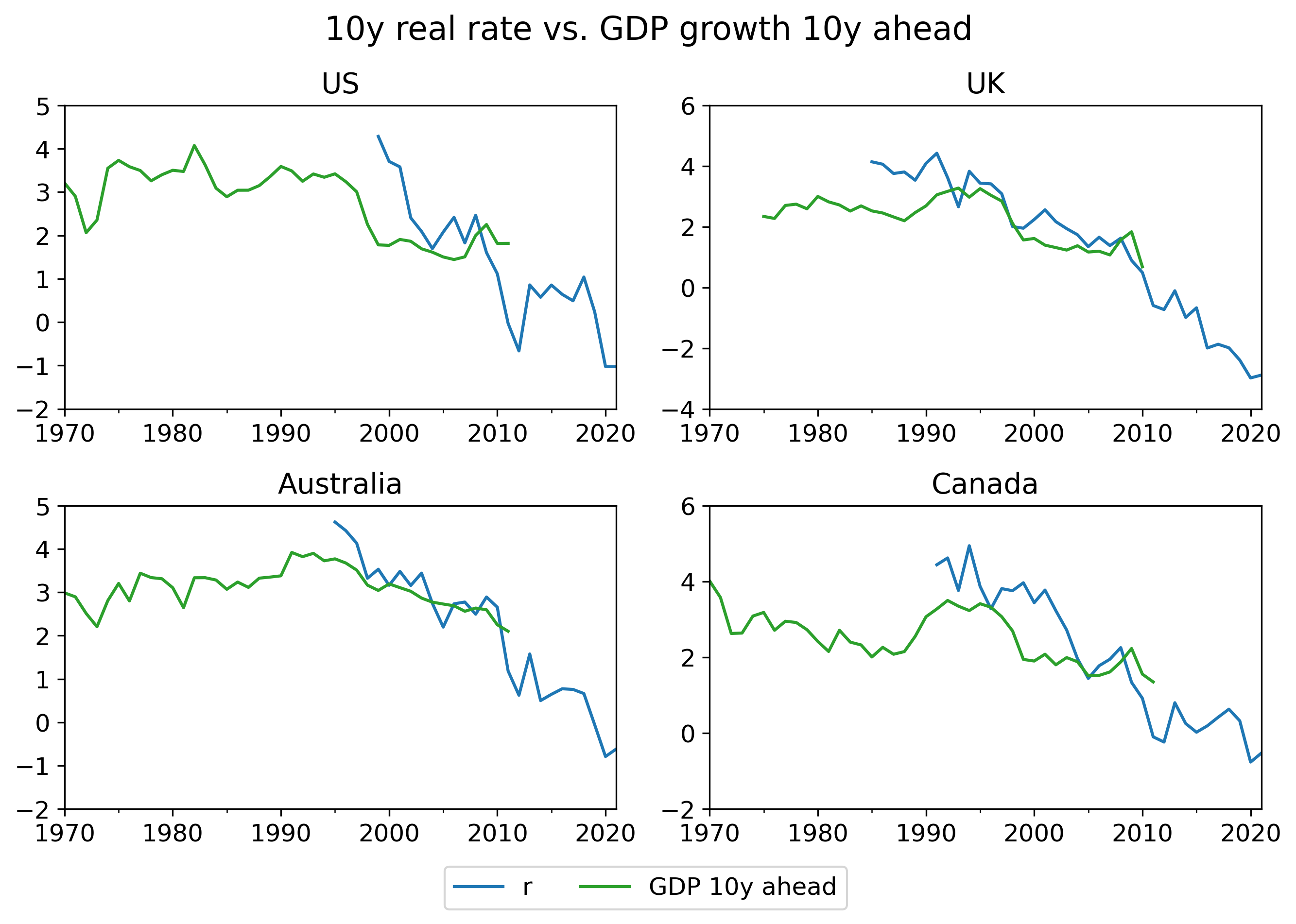
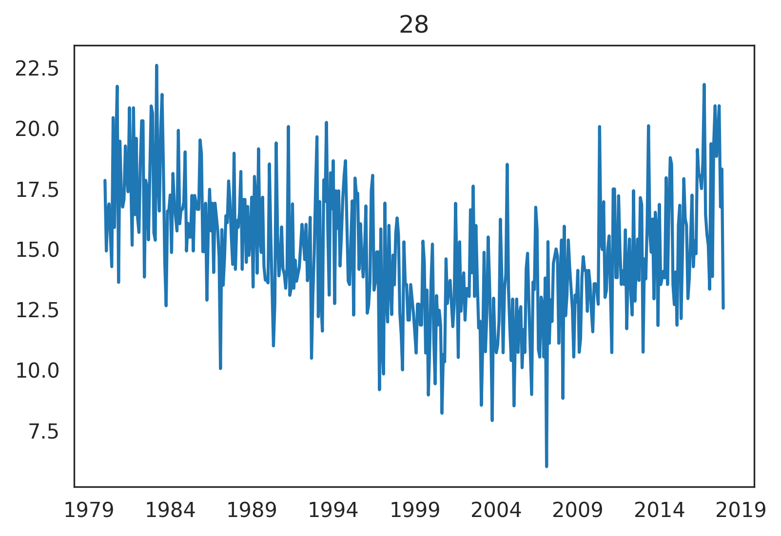
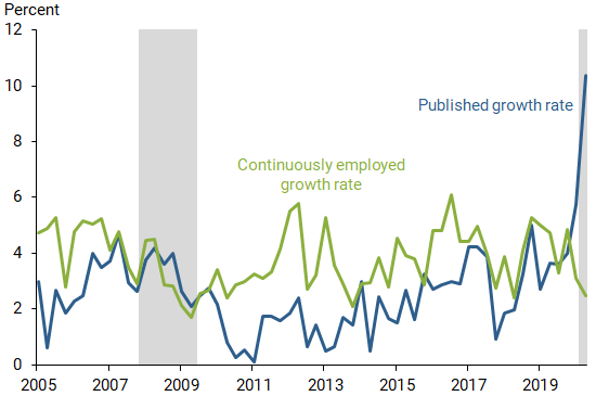